BCB 520 - Final Project

Project Description:

Understanding Bighorn Sheep Nutrition and Movement in the John Day Canyon

Located within the Columbia Plateau, the John Day Canyon is a steep, rugged landscape where sagebrush and grasses dominate the hillsides. This dynamic environment supports a unique population of bighorn sheep — one that, remarkably, has avoided the disease outbreaks that often devastate other herds.

My research focuses on understanding the nutritional requirements of these bighorn sheep and how those needs shift throughout their reproductive cycle due to changing metabolic demands. The ultimate goal is to develop a predictive model that links their nutritional requirements to movement patterns. By doing so, we can identify potential threats, such as areas where bighorn sheep may come into contact with domestic livestock, and pinpoint critical habitats essential for their survival.

To achieve this, I am collecting vegetation data to calculate a measure of “suitable biomass”—essentially, the portion of available forage that meaningfully contributes to the sheep’s energy needs at different reproductive stages. This metric is created using measures of digestible energy and digestible protein. I have currently not finalized my values of “suitable biomass”, but I do have preliminary values of digestible energy and digestible protein from a subset of my data. Eventually using this metric, I will develop a Generalized Additive Model (GAM) to map areas of high and low nutritional quality across the landscape.

These techniques will help determine which resources most influence bighorn sheep movement and allow us to predict future movement patterns—a critical step in ensuring their continued success in this landscape. By bridging nutritional ecology with movement ecology, this research will contribute valuable insights into how bighorn sheep navigate their environment and help inform conservation strategies for this unique, disease-free population.

Data Wrangling

library(lpSolve)
library(openxlsx)
library(tools)
library(dplyr)
library(sf)
library(tidyverse)

# Define the path to the directory containing the file
excelpath <- "C:/Users/Alexis Means/Documents/Project/Nutrition Sampling/R code/FRESH/processed.data/"

# Define the specific file name
filename <- "FRESH.Subset.xlsx"

# Construct the full file path
excel.file <- file.path(excelpath, filename)

# Load the workbook and read the data
library(openxlsx)
habitat <- loadWorkbook(excel.file)
data <- data.frame(readWorkbook(excel.file, sheet = "FRESH Data", startRow = 1, colNames = TRUE))


plant <-read.csv("C:/Users/Alexis Means/Documents/Project/Nutrition Sampling/R code/Cleaning/processed.data/plant.csv")

data <- data %>% 
  rename(Code = Plant.Code) %>% 
  left_join(y = plant, 
            by = "Code",
            relationship = "many-to-one")

Data Dictionary

For further description as to what each of my variables are within my data set. Please see my data dictionary here.

table<- read.csv("C:/Users/Alexis Means/Documents/School/BCB520/2A/attributes.csv") 
knitr::kable(table)

Attribute	Type	Note
Biomass	Quantitative	This measurement tells us what the weight of dry biomass is for each specific observation
TransectID	Categorical	This descriptor is a unique ID that tells us which randomized point we sampled
Quadrat	Categorical	There are 5 quadrats that we sample for each quadrat (20,40,60,80,100)
Code	Categorical	These are unique codes that describe the family, genius and species for every item observed
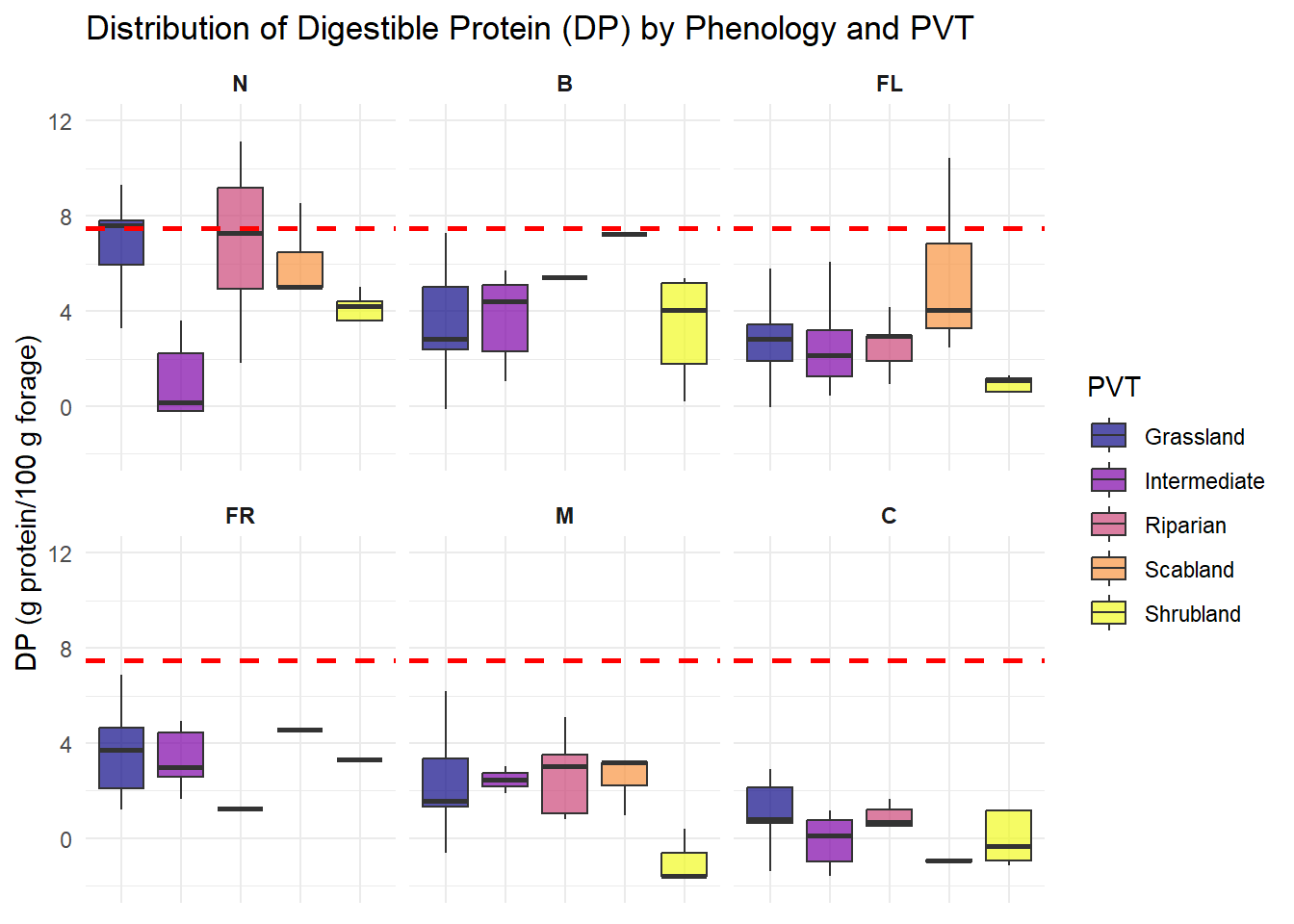
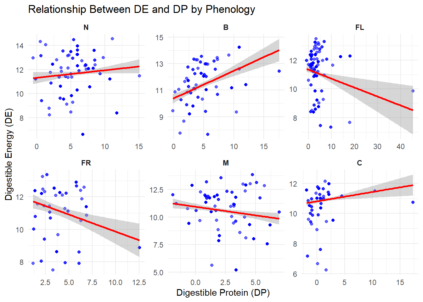
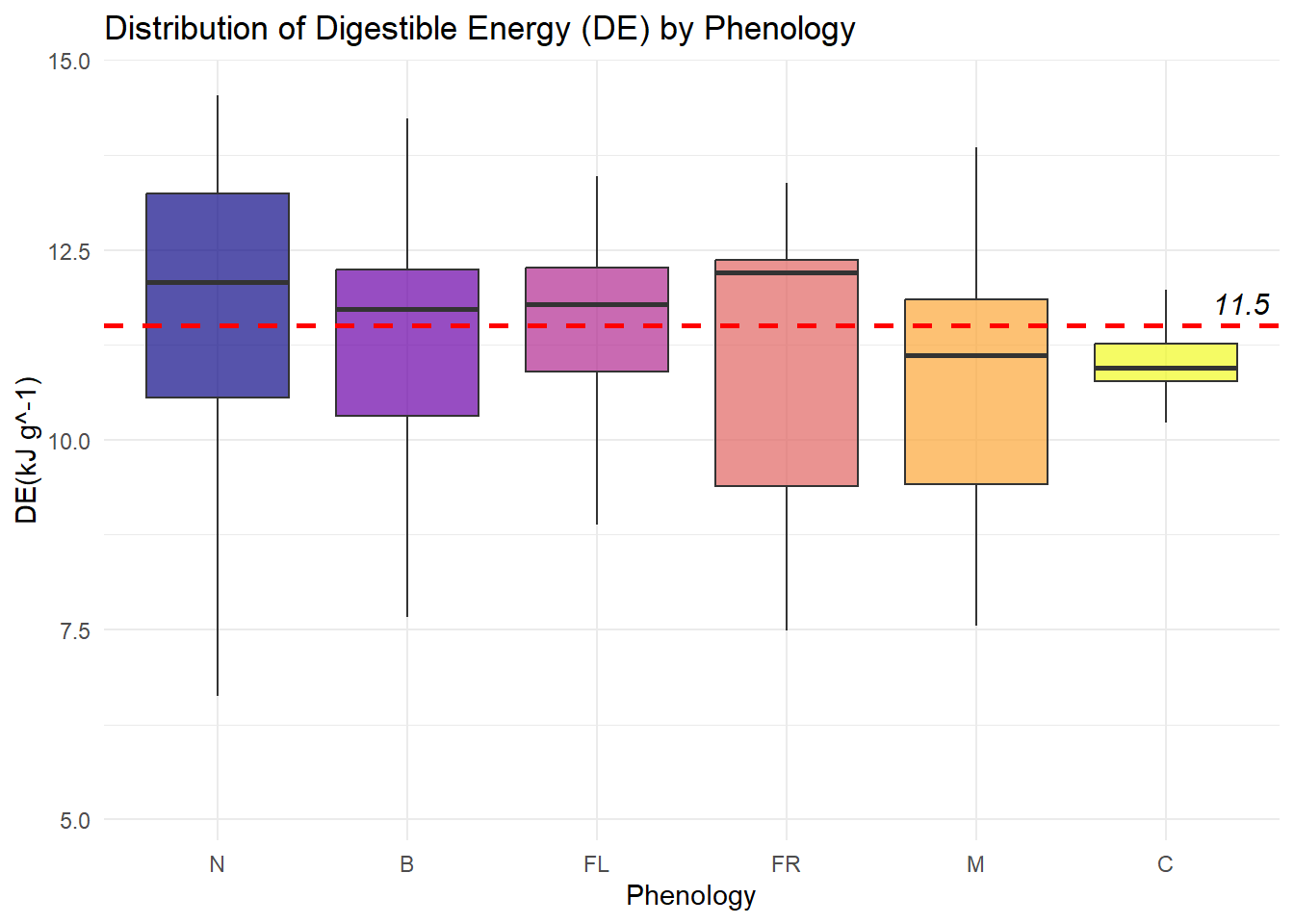
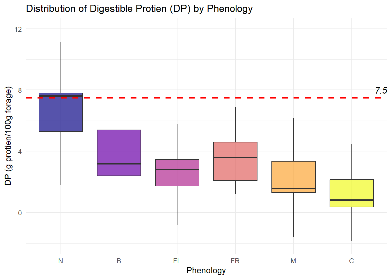
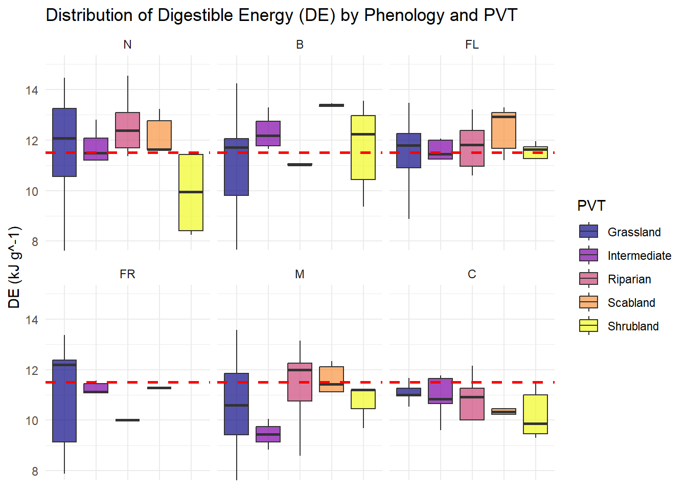
Phenology	Categorical	Each species is assigned a growth stage when we observe it - New, Budding, Flowering, Fruiting, Mature or Cured (N, B, FL, FR, M, C)
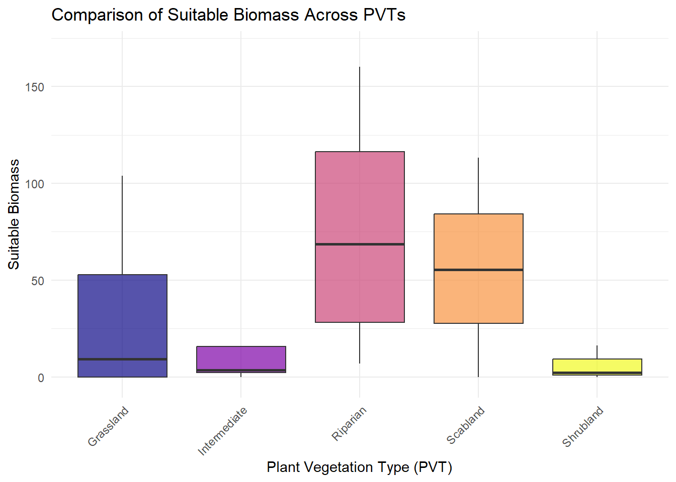
PVT	Categorical	This number describes the vegetation community that was being sampled, we have 5 total for the study area, it is used as part of the descriptor for each plotID
percent	Quantitative	This measurement tells us the percent cover that each composition_id occupies within a 1x1m quadrat
Spp	Categorical	This unique ID is slightly more broad and will be used to identify species/phenology combinations within each vegetation type as well as the season
Family	Categorical	This will be used to group quality data if we do not have enough information to determine the quality down to the smaller scale (genus)
Genus	Categorical	This will be used to group quality data if we do not have enough information to determine the quality down to the smaller scale (spp)
Species	Categorical	This will be used to group quality data if we do not have enough information to determine the quality down to the smaller scale (phenological stage)
FunctionalGroup	Categorical	The smallest grouping variable for my quality data (perennial or annual grass, forb, or shrub)
FGNew	Categorical	Shortened version of FunctionalGroup
CommonName	Categorical	This is another identifier for each species, it will likely not be used within the analysis so it could be removed
Duration	Categorical	This is another category I may use to group quality data based on the growth duration of each species
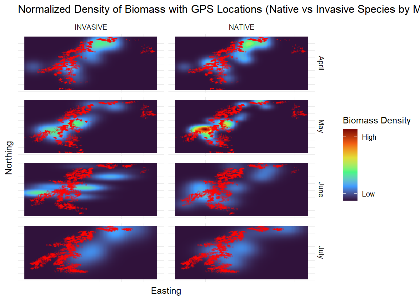
Status	Categorical	Each species is categorized as native or invasive
Season	Categorical	Our observations are grouped based on the date that they were sampled (Spring, Summer and Fall) to observe the changes in nutritional quality
Dates	Categorical	This keeps track of the day that each observation was sampled
Aspect	Categorical	Described the direction the hill was facing that each of our transects had been sampled on
Elev	Quantitative	Describes the elevation that each of the transects was sampled at
Lat/Long	Categorical	Each of the lat/long pairs plots the beginning, middle and end of each of the transects
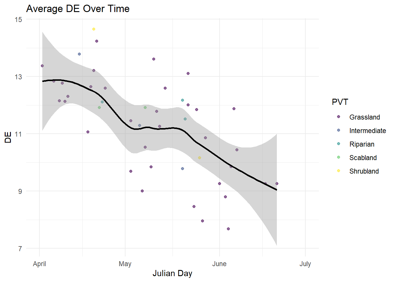
DE	Quantitative	Amount of digestible energy provided by each species
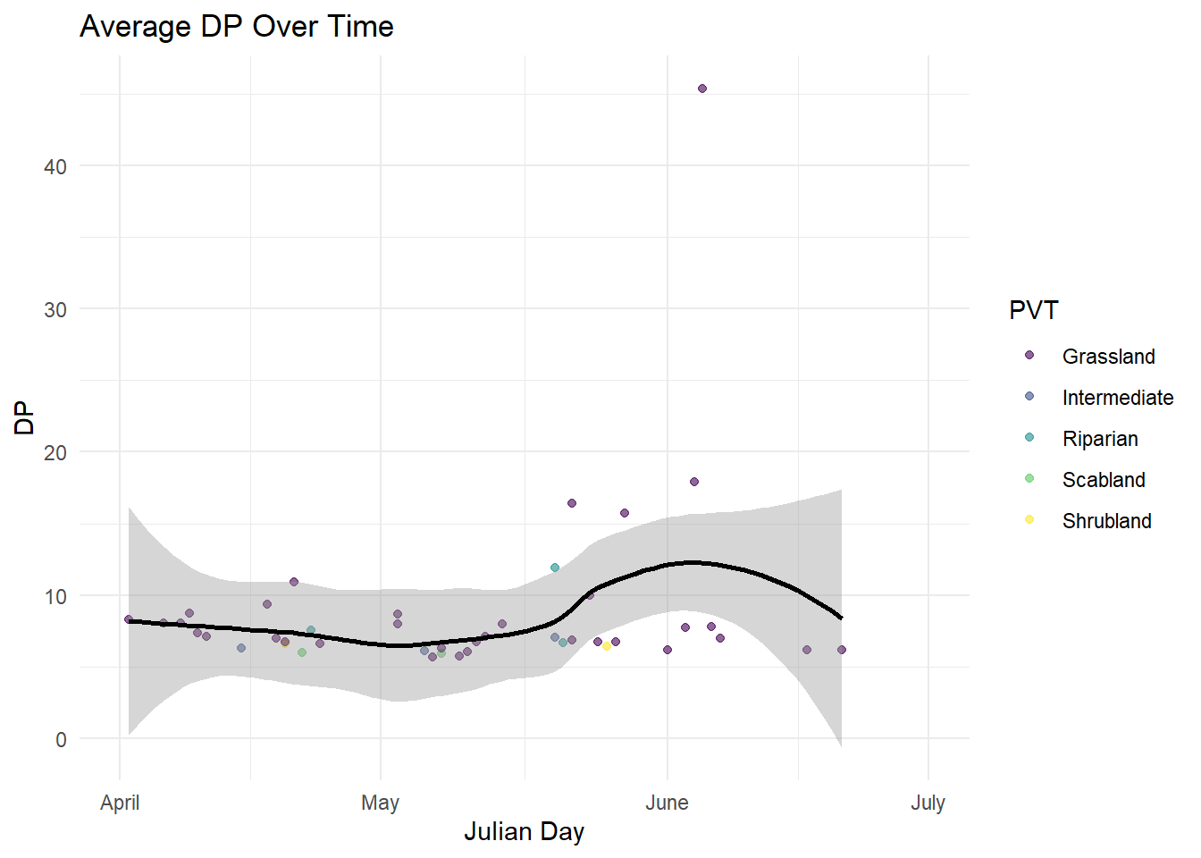
DP	Quantitative	Amount of digestible protien provided by each species
DE.SD	Quantitative	Standard deviation of digestible energy
DP.SD	Quantitative	Standard deviation of digestible protien
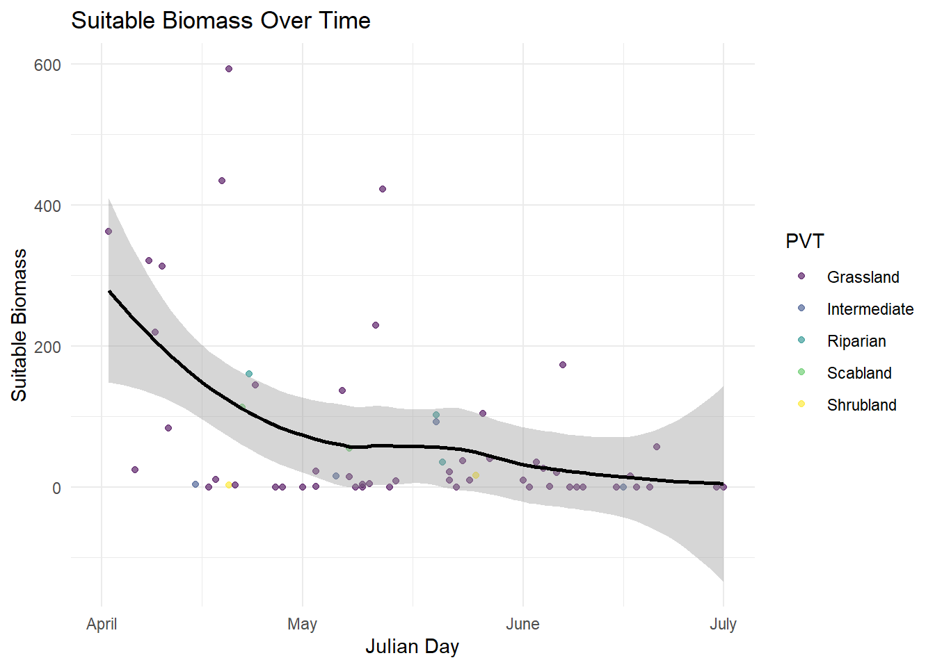
Julian Date	Categorical	The converted date that each of the plots was sampled to julian day
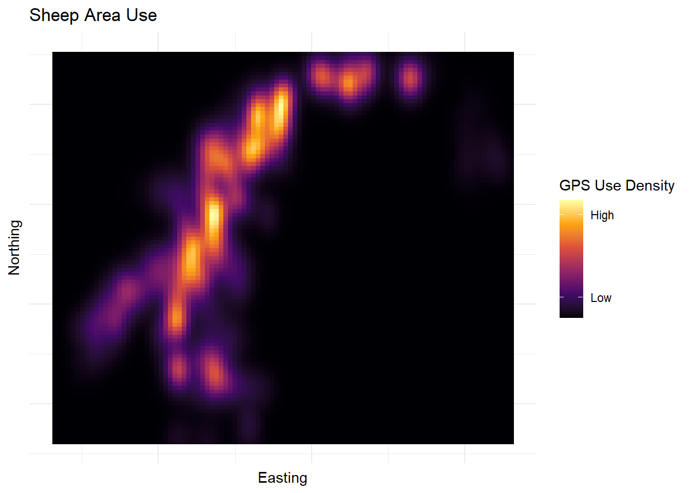
Easting	Categorical	The converted latitude to UTM
Northing	Categorical	The converted longitude to UTM
TotalDE	Quantitative	The amount of total DE available at a transect
TotalDP	Quantitative	The amount of total DP available at a transect
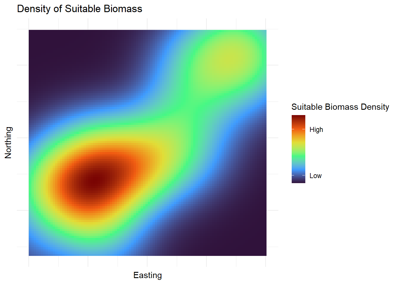
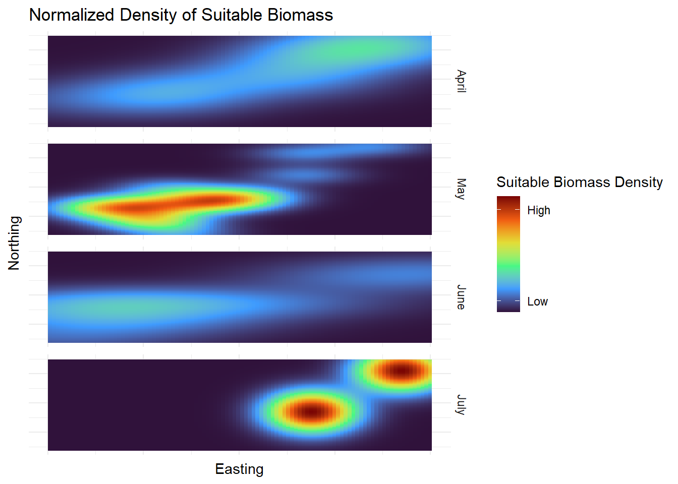
SuitableBiomass	Quantitative	The amount of forage available at each transect that meet the assigned energetic demands of a lactating female sheep
AveDE	Quantitative	The average amount of digestible energy available at a transect
AveDP	Quantitative	The average amount of digestible protien available at a transect
Month	Categorical	The month that the plot was sampled

Exploring Quality Trends

Comparing DE and DP values for phenological stage

Using a subset of my quality data, I began by comparing measurements of digestible energy (DE) and digestible protein (DP) across plant species and phenological stages. My main goal was to explore whether there is a correlation between high DE and high DP. The scatter plot results showed a pattern consistent with my expectations: the highest values for both DE and DP occur during the newly emergent (N) and budding (B) stages. These values drop sharply by the flowering (FL) stage and remain relatively stable thereafter.

library(tidyverse)

data$Phenology <- factor(data$Phenology, levels = c("N", "B", "FL", "FR", "M", "C"))

ggplot(data, aes(x = DP, y = DE)) +
  geom_point(color = "blue", alpha = 0.6) +
  geom_smooth(method = "lm", se = TRUE, color = "red") + 
  labs(title = "Relationship Between DE and DP by Phenology",
       x = "Digestible Protein (DP)",
       y = "Digestible Energy (DE)") +
  theme_minimal() +
  facet_wrap(~ Phenology, scales = "free") +
  scale_x_continuous(expand = c(0.05, 0)) +  
  scale_y_continuous(expand = c(0.05, 0)) +
  theme(strip.text = element_text(face = "bold"))  

To better visualize the trends in DP and DE across phenological stages, I isolated the DE and DP values for direct comparison. Both metrics follow the expected pattern, showing a general decline over progressing phenological stage. While many species meet the DE requirement of 11.5 kJ per gram of forage, very few meet the necessary DP threshold of 7.5 g per 100 g of forage beyond the newly emergent stage. These thresholds represent the minimum forage quality needed to meet the energetic and protein demands of a lactating female sheep.

# Ensure Phenology is a factor with the correct order
data$Phenology <- factor(data$Phenology, levels = c("N", "B", "FL", "FR", "M", "C"))

ggplot(data, aes(x = Phenology, y = DE, fill = Phenology)) +
  geom_boxplot(alpha = 0.7, outlier.shape = NA) +  
  scale_fill_viridis_d(option = "plasma") +  
  labs(title = "Distribution of Digestible Energy (DE) by Phenology",
       x = "Phenology",
       y = "DE(kJ g^-1)") +
  theme_minimal() +
  theme(legend.position = "none")+
   geom_hline(yintercept = 11.5, linetype = "dashed", color = "red", size = 1)+
  annotate("text", x = 6.4, y = 11.8, label = "11.5", color = "black", size = 4, fontface = "italic")

ggplot(data, aes(x = Phenology, y = DP, fill = Phenology)) +
  geom_boxplot(alpha = 0.7, outlier.shape = NA) +  
  scale_fill_viridis_d(option = "plasma") +  
  labs(title = "Distribution of Digestible Protien (DP) by Phenology",
       x = "Phenology",
       y = "DP (g protien/100g forage)") +
  theme_minimal() +
  theme(legend.position = "none")+
   geom_hline(yintercept = 7.5, linetype = "dashed", color = "red", size = 1)+
  annotate("text", x = 6.5, y = 8, label = "7.5", color = "black", size = 4, fontface = "italic")+
  coord_cartesian(ylim = c(-2, 12))

Quality Metrics Compared across Vegetation Type

I was curious whether this trend varied across different vegetation types, particularly in riparian areas, which retain the most moisture. However, I did not observe any clear pattern indicating that a specific vegetation type consistently supported significantly higher quality metrics than others.

data <- data %>%
  mutate(PVT = str_sub(TransectID, start = 4, end = 6)) %>% 
  group_by(PVT) %>%
  mutate(Stand_DE = scale(DE)) %>%
  mutate(Stand_DP = scale(DP)) %>%
  ungroup()

data <- data %>%
  mutate(PVT = case_when(
    PVT == "672" ~ "Grassland",
    PVT == "682" ~ "Riparian",
    PVT == "674" ~ "Intermediate",
    PVT == "668" ~ "Scabland",
    PVT == "669" ~ "Shrubland",
    TRUE ~ as.character(PVT)  # This keeps any other values unchanged
  ))

ggplot(data, aes(x = PVT, y = DE, fill = PVT)) +
  geom_boxplot(alpha = 0.7, outlier.shape = NA) +  
  scale_fill_viridis_d(option = "plasma") +  
  labs(title = "Distribution of Digestible Energy (DE) by Phenology and PVT",
       x = NULL,  # Remove x-axis label
       y = "DE (kJ g^-1)",
       fill = "PVT") +  # Label for the legend
  theme_minimal() +
  theme(
    legend.position = "right",  # Show legend on the right
    axis.text.x = element_blank(),  # Remove x-axis text
    axis.ticks.x = element_blank()  # Remove x-axis ticks
  ) +
  geom_hline(yintercept = 11.5, linetype = "dashed", color = "red", size = 1) +
  facet_wrap(~ Phenology, scales = "free_x", ncol = 3) +
  coord_cartesian(ylim = c(8, 15))

ggplot(data, aes(x = PVT, y = DP, fill = PVT)) +
  geom_boxplot(alpha = 0.7, outlier.shape = NA) +  
  scale_fill_viridis_d(option = "plasma") +  
  labs(title = "Distribution of Digestible Protein (DP) by Phenology and PVT",
      x = NULL,  # Remove x-axis label
       y = "DP (g protein/100 g forage)",
       fill = "PVT") +  # Label for the legend
  theme_minimal() +
  theme(legend.position = "right",  # Show legend on the right
    axis.text.x = element_blank(),  # Remove x-axis text
    axis.ticks.x = element_blank(),
    strip.text = element_text(face = "bold")# Remove x-axis ticks
  ) +
  geom_hline(yintercept = 7.5, linetype = "dashed", color = "red", size = 1) +
  facet_wrap(~ Phenology, scales = "free_x", ncol = 3)+
  coord_cartesian(ylim = c(-2, 12))

plot <- read.csv("C:/Users/Alexis Means/Documents/Project/Nutrition Sampling/R code/Cleaning/processed.data/transect.csv")

# Define the path to the directory containing the file
excelpath <- "C:/Users/Alexis Means/Documents/Project/Nutrition Sampling/R code/FRESH/processed.data/"

# Define the specific file name
filename <- "2024.subset.results.xlsx"

# Construct the full file path
excel.file <- file.path(excelpath, filename)

# Load the workbook and read the data

habitat <- loadWorkbook(excel.file)
suitable <- data.frame(readWorkbook(excel.file, sheet = "Plot-Level-Summary", startRow = 1, colNames = TRUE))


suitable <- suitable %>% 
  rename(PlotID = TransectID) %>% 
  left_join(y = plot,
            by = "PlotID")

suitable <- suitable %>% 
  rename(Lat = BeginLat,
         Long = BeginLong,
         Easting = BeginUTM_Easting,
         Northing = BeginUTM_Northing) %>% 
  select(PlotID, TotalDE, TotalDP, SuitableBiomass, AveDE, AveDP, Julian_Day, Lat, Long, Easting, Northing)


# Create an sf object with the Lat and Long columns
suitable_UTM <- st_as_sf(suitable, coords = c("Long", "Lat"), crs = 4326)  # EPSG:4326 is WGS84

# Convert to UTM Zone 11N (EPSG:26911)
suitable_UTM <- st_transform(suitable_UTM, crs = 32611)

# Extract UTM coordinates (Easting and Northing)
suitable$Easting <- st_coordinates(suitable_UTM)[, 1]
suitable$Northing <- st_coordinates(suitable_UTM)[, 2]

suitable <- suitable %>%  
mutate(Month = case_when(
    Julian_Day >= 93 & Julian_Day < 124 ~ "April",
    Julian_Day >= 124 & Julian_Day < 155 ~ "May",
    Julian_Day >= 155 & Julian_Day < 185 ~ "June",
    Julian_Day >= 185 & Julian_Day <= 212 ~ "July",
    TRUE ~ NA_character_
  )) %>%
  filter(!is.na(Month)) %>%
  mutate(Month = factor(Month, levels = c("April", "May", "June", "July")))

suitable <- suitable %>% 
  mutate(PVT = str_sub(PlotID, start = 4, end = 6)) %>% 
  mutate(PVT = case_when(
    PVT == "672" ~ "Grassland",
    PVT == "682" ~ "Riparian",
    PVT == "674" ~ "Intermediate",
    PVT == "668" ~ "Scabland",
    PVT == "669" ~ "Shrubland",
    TRUE ~ as.character(PVT)  # This keeps any other values unchanged
  ))

Suitable Biomass by Vegetation Type

Using measurements of DE and DP, along with the biomass of forage collected at my transects, I applied the FRESH Model (Hanley et al. 2012) to evaluate how many of the sampled areas met the nutritional requirements of a lactating female sheep, based on the combined contribution of all observed species. This analysis produced my estimate of “suitable biomass.”

While my initial hypothesis was that riparian areas would stand out for their nutrient quality, this was not supported by the DE and DP values alone. However, due to the higher plant density in these moisture-rich areas, riparian zones did yield a much greater total biomass, resulting in higher suitable biomass values overall compared to other vegetation types.

One vegetation community that caught my attention was the scabland community. Found mostly on exposed ridges, these areas are typically rocky, wind-swept, and sun-exposed—conditions not usually associated with high productivity. However, these ridges are often the most accessible points in the landscape and are frequently used by landowners for grazing cattle on BLM land. They also lie closer to potential sources of agricultural runoff and experience more frequent disturbance. I suspect that these human influences may be altering the natural composition and productivity of the scabland community. Therefore, I plan to include distance to private land as a variable in my GAM, as I believe it may be a key factor shaping this vegetation type.

ggplot(suitable, aes(x = PVT, y = SuitableBiomass, fill = PVT)) +
  geom_boxplot(alpha = 0.7, outlier.shape = NA) +
  scale_fill_viridis_d(option = "plasma") +
  labs(title = "Comparison of Suitable Biomass Across PVTs",
       x = "Plant Vegetation Type (PVT)",
       y = "Suitable Biomass") +
  theme_minimal() +
  theme(legend.position = "none",
        axis.text.x = element_text(angle = 45, hjust = 1))+
  coord_cartesian(ylim = c(-2, 170))

Quality Trends overtime

Next, I looked at how these forage quality metrics changed over time. It’s important to note that if a transect did not meet the nutritional requirements for a lactating female sheep, it was assigned a suitable biomass value of zero. Because of this, it may appear that my sampling ended in early July, even though I continued collecting data through August. This is likely because many transects no longer met the nutritional thresholds by mid-summer, resulting in more zeros for suitable biomass.

The trends in suitable biomass and digestible energy align with my expectations—they both decline over time. Digestible protein, however, remains relatively stable throughout the season.

It’s also reassuring to see that my assumption about the timing of the “green-up”—the period when forage is at its most nutritious—was accurate. The first graph shows a steady decline in suitable biomass until mid-May, after which values remain fairly constant with only a slight decrease through the rest of the summer.

# Define the Julian days and corresponding month labels
date_breaks <- c(92, 122, 155, 185)
date_labels <- c("April", "May", "June", "July")


ggplot(suitable, aes(x = Julian_Day, y = SuitableBiomass)) +
  geom_point(aes(color = PVT), alpha = 0.6) +
  geom_smooth(method = "loess", se = TRUE, color = "black") +
  scale_color_viridis_d() +
  labs(title = "Suitable Biomass Over Time",
       x = "Julian Day",
       y = "Suitable Biomass",
       color = "PVT") +
  theme_minimal() +
  theme(legend.position = "right",
        axis.text.x = element_text(angle = 0, hjust = 0.5)) +
  scale_x_continuous(breaks = date_breaks,
    labels = date_labels,
    limits = c(min(date_breaks), max(date_breaks))
  )

ggplot(suitable, aes(x = Julian_Day, y = AveDE)) +
  geom_point(aes(color = PVT), alpha = 0.6) +
  geom_smooth(method = "loess", se = TRUE, color = "black") +
  scale_color_viridis_d() +
  labs(title = "Average DE Over Time",
       x = "Julian Day",
       y = "DE",
       color = "PVT") +
  theme_minimal() +
  theme(legend.position = "right",
        axis.text.x = element_text(angle = 0, hjust = 0.5)) +
  scale_x_continuous(breaks = date_breaks,
    labels = date_labels,
    limits = c(min(date_breaks), max(date_breaks))
  )

ggplot(suitable, aes(x = Julian_Day, y = AveDP)) +
  geom_point(aes(color = PVT), alpha = 0.6) +
  geom_smooth(method = "loess", se = TRUE, color = "black") +
  scale_color_viridis_d() +
  labs(title = "Average DP Over Time",
       x = "Julian Day",
       y = "DP",
       color = "PVT") +
  theme_minimal() +
  theme(legend.position = "right",
        axis.text.x = element_text(angle = 0, hjust = 0.5)) +
  scale_x_continuous(
    breaks = date_breaks,
    labels = date_labels,
    limits = c(min(date_breaks), max(date_breaks))
  )

Biomass Trends

One of the key parts of my project is understanding the spread of invasive species throughout the canyon, specifically cheat grass. When observing the canyon it seems like cheat grass dominates the landscape which could effect the amount of nutrients available later in the summer after much of it has progressed through its flowering stage. To start I wanted to looks at the density of biomass for all native versus invasive species within the transects that I sampled in our study area. From this graph we can see that overall biomass of native and invasive species is relatively similar throughout the canyon. However, there is an overall greater density of native species.

spp.map <- data %>% 
  select(TransectID, Code, Phenology, Part, Biomass, Duration, Status)

plot <- read.csv("C:/Users/Alexis Means/Documents/Project/Nutrition Sampling/R code/Cleaning/processed.data/transect.csv")

spp.map <- spp.map %>% 
  rename(PlotID = TransectID)

spp.map <- spp.map %>% 
  left_join(y = plot,
            by = "PlotID",
            relationship = "many-to-one")

spp.map <- spp.map %>% 
  rename(Lat = BeginLat,
         Long = BeginLong,
         Easting = BeginUTM_Easting,
         Northing = BeginUTM_Northing) %>% 
  select(PlotID, Code, Phenology, Part, Biomass, Duration, Status, Julian_Day, Lat, Long, Easting, Northing)


# Create an sf object with the Lat and Long columns
spp.map_UTM <- st_as_sf(spp.map, coords = c("Long", "Lat"), crs = 4326)  # EPSG:4326 is WGS84

# Convert to UTM Zone 11N (EPSG:26911)
spp.map_UTM <- st_transform(spp.map_UTM, crs = 32611)

# Extract UTM coordinates (Easting and Northing)
spp.map$Easting <- st_coordinates(spp.map_UTM)[, 1]
spp.map$Northing <- st_coordinates(spp.map_UTM)[, 2]

# Load necessary libraries
library(tidyverse)

# Summarize biomass weight by spatial location and species status
spp.summary <- spp.map %>%
   filter(!is.na(Biomass) & Biomass > 0)  # Remove NAs
  
ggplot(spp.summary, aes(x = Easting, y = Northing, weight = Biomass)) +
  stat_density_2d(aes(fill = after_stat(density)), geom = "raster", contour = FALSE) +
  facet_wrap(~ Status) +  # Separate maps for Native/Invasive
  scale_fill_viridis_c(
    name = "Biomass Density", 
    option = "turbo",
    breaks = c(1e-09, 7e-09),  # Define specific density values
    labels = c("Low", "High")  # Replace numerical values with "Low" and "High"
  ) +  
  labs(title = "Density of Biomass (Native vs Invasive Species)",
       x = "Easting", 
       y = "Northing") +
  theme_minimal() +
  theme(axis.text = element_blank(),  # Remove tick labels
    axis.ticks = element_blank())  # Rotate x-axis labels

I am still currently using only a subset of my quality data, so these results may be slightly skewed from the results of my complete data set.

I would also like to see the differences in overall biomass for each month. I had a much larger sample size in April and May than I did in June and July, so I standardized my biomass values before plotting them.

month.sum <- spp.map %>%
  filter(!is.na(Biomass) & Biomass > 0) %>%  # Remove NAs
  mutate(Month = case_when(
    Julian_Day >= 93 & Julian_Day < 124 ~ "April",
    Julian_Day >= 124 & Julian_Day < 155 ~ "May",
    Julian_Day >= 155 & Julian_Day < 185 ~ "June",
    Julian_Day >= 185 & Julian_Day <= 212 ~ "July",
    TRUE ~ NA_character_
  )) %>%
  filter(!is.na(Month)) %>%
  mutate(Month = factor(Month, levels = c("April", "May", "June", "July")))

# Normalize biomass within each month (to make sample sizes comparable)
month.sum <- month.sum %>%
  group_by(Month) %>%
  mutate(Total_Biomass = sum(Biomass),  # Calculate total biomass for each month
         Normalized_Biomass = Biomass / Total_Biomass) %>%  # Normalize biomass
  ungroup()  # Remove grouping


# Create density plot faceted by Month and Status
ggplot(month.sum, aes(x = Easting, y = Northing, weight = Normalized_Biomass)) +
  stat_density_2d(aes(fill = after_stat(density)), geom = "raster", contour = FALSE) +
  facet_grid(Month ~ Status) +  # Grid facet by Month (rows) and Status (columns)
  scale_fill_viridis_c(
    name = "Biomass Density", 
    option = "turbo",
    breaks = c(2e-09, 18e-09),  # Define specific density values
    labels = c("Low", "High")  # Replace numerical values with "Low" and "High"
  ) +  
  labs(title = "Normalized Density of Biomass (Native vs Invasive Species by Month)",
       x = "Easting", 
       y = "Northing") +
  theme_minimal() +
  theme(axis.text = element_blank(),  # Remove tick labels
        axis.ticks = element_blank())

Since cheatgrass is the main invasive species we’ve been tracking in the canyon, I’m especially interested in how its biomass changes from month to month. In this part of my dataset, I didn’t record any cheatgrass observations in June, so I’ll need to be cautious about interpreting the rest of the results until I can finish my biomass predictions. That said, the data I do have suggest that cheatgrass biomass peaked in the southern end of the canyon around June and began to decline after that.

# Filter for observations with Species Code "BRTE"
cheat.sum <- spp.map %>%
  filter(!is.na(Biomass) & Biomass > 0, Code == "BRTE") %>%  # Remove NAs and filter for "BRTE"
  mutate(Month = case_when(
    Julian_Day >= 93 & Julian_Day < 124 ~ "April",
    Julian_Day >= 124 & Julian_Day < 155 ~ "May",
    Julian_Day >= 155 & Julian_Day < 185 ~ "June",
    Julian_Day >= 185 & Julian_Day <= 212 ~ "July",
    TRUE ~ NA_character_
  )) %>%
  filter(!is.na(Month)) %>%
  mutate(Month = factor(Month, levels = c("April", "May", "June", "July")))  # Set correct order

# Normalize biomass within each month (to make sample sizes comparable)
cheat.sum <- cheat.sum %>%
  group_by(Month) %>%
  mutate(Total_Biomass = sum(Biomass),  # Calculate total biomass for each month
         Normalized_Biomass = Biomass / Total_Biomass) %>%  # Normalize biomass
  ungroup()  # Remove grouping

# Create density plot faceted by Month and Status for species "BRTE"
ggplot(cheat.sum, aes(x = Easting, y = Northing, weight = Normalized_Biomass)) +
  stat_density_2d(aes(fill = after_stat(density)), geom = "raster", contour = FALSE) +
  facet_grid(Month ~ Code) +  # Grid facet by Month (rows) and Status (columns)
  scale_fill_viridis_c(
    name = "Biomass Density", 
    option = "turbo",
    breaks = c(2e-09, 14e-09),  # Define specific density values
    labels = c("Low ", "High ")  # Replace numerical values with "Low" and "High"
  ) +  
  labs(title = "Normalized Density of Biomass for BRTE by month",
       x = "Easting", 
       y = "Northing") +
  theme_minimal() +
  theme(axis.text = element_blank(),  # Remove tick labels
        axis.ticks = element_blank())

The metric of “suitable biomass” is a single value applied to my transect, so I have not figured out how to apply that value to specific species. I could however look at the overall DE and DP for native versus invasive species. (another graph to add to the to-do list)

GPS Data

Lastly, I want to see how the sheep movements change each month with the overall biomass of both native and invasive species. I started out by creating a heat map of our overall sheep location use throughout the canyon.

gps <- read.csv("C:/Users/Alexis Means/Documents/Project/Demographics/Code/cleaned.data/sheep_clean_24.csv")

gps <- gps %>% 
  rename(Easting = x_,
         Northing = y_)

# Step 1: Kernel Density Estimation (KDE) for GPS data
gps_kde <- ggplot(gps, aes(x = Easting, y = Northing)) +
  stat_density_2d(aes(fill = after_stat(density)), geom = "raster", contour = FALSE) +
  scale_fill_viridis_c(option = "inferno",
          name = "GPS Use Density",
          breaks = c(2e-09, 10e-09),  # Define specific density values
          labels = c("Low", "High")  # Replace  values with "Low" and "High"
  ) +
  labs(title = "Sheep Area Use")+
  theme_minimal()+
  theme(axis.text = element_blank(),  # Remove tick labels
        axis.ticks = element_blank()) 
  plot(gps_kde)

If the areas of high biomass density align with values of high nutrient quality in theory this means that the density of our sheep points should also follow the trends of high biomass density in the months of April and May. I wanted to see if I could overlay our sheep locations each month with the biomass density data each month to observe my hunch that sheep would follow this trend in these months. They do not appear to follow this trend, most likely due to other outside factors such as selection for escape terrain that outweigh the need to follow vegetation trends. It is also likely that areas of high biomass does not always mean areas of high nutritional quality.

month.sum <- spp.map %>%
  filter(!is.na(Biomass) & Biomass > 0) %>%  # Remove NAs
  mutate(Month = case_when(
    Julian_Day >= 93 & Julian_Day < 124 ~ "April",
    Julian_Day >= 124 & Julian_Day < 155 ~ "May",
    Julian_Day >= 155 & Julian_Day < 185 ~ "June",
    Julian_Day >= 185 & Julian_Day <= 212 ~ "July",
    TRUE ~ NA_character_
  )) %>%
  filter(!is.na(Month)) %>%
  mutate(Month = factor(Month, levels = c("April", "May", "June", "July")))


# Normalize biomass within each month (to make sample sizes comparable)
month.sum <- month.sum %>%
  group_by(Month) %>%
  mutate(Total_Biomass = sum(Biomass),  # Calculate total biomass for each month
         Normalized_Biomass = Biomass / Total_Biomass) %>%  # Normalize biomass
  ungroup()  # Remove grouping

# Extract month from the GPS timestamp
gps <- gps %>%
  mutate(Month = case_when(
    month(t_) == 4 ~ "April",
    month(t_) == 5 ~ "May",
    month(t_) == 6 ~ "June",
    month(t_) == 7 ~ "July",
    TRUE ~ NA_character_
  )) %>%
  filter(!is.na(Month)) %>% 
  mutate(Month = factor(Month, levels = c("April", "May", "June", "July")))

ggplot() + # Biomass density heatmap using kernel density estimation
  stat_density_2d(
    data = month.sum,
    aes(x = Easting, y = Northing, weight = Normalized_Biomass, fill = after_stat(density)),
    geom = "raster",
    contour = FALSE
  ) +
  facet_grid(Month ~ Status) +  # Grid facet by Month (rows) and Status (columns)
  scale_fill_viridis_c(
    name = "Biomass Density", 
    option = "turbo",
    breaks = c(2e-09, 18e-09),  # Define specific density values
    labels = c("Low", "High")  # Replace numerical values with "Low" and "High"
  ) +  
  labs(title = "Normalized Density of Biomass with GPS Locations (Native vs Invasive Species by Month)",
       x = "Easting", 
       y = "Northing") +
  theme_minimal() +
  theme(axis.text = element_blank(),  # Remove tick labels
        axis.ticks = element_blank()) +
  # Overlay GPS points, filtering by Month to match the facet
  geom_point(
    data = gps, 
    aes(x = Easting, y = Northing), 
    color = "red", alpha = 0.1, size = 0.4
  )

# Define the path to the directory containing the file
excelpath <- "C:/Users/Alexis Means/Documents/Project/Nutrition Sampling/R code/FRESH/processed.data/"

# Define the specific file name
filename <- "2024.subset.results.xlsx"

# Construct the full file path
excel.file <- file.path(excelpath, filename)

# Load the workbook and read the data

habitat <- loadWorkbook(excel.file)
suitable <- data.frame(readWorkbook(excel.file, sheet = "Plot-Level-Summary", startRow = 1, colNames = TRUE))


suitable.map <- suitable %>% 
  rename(PlotID = TransectID) %>% 
  left_join(y = plot,
            by = "PlotID")

suitable.map <- suitable.map %>% 
  rename(Lat = BeginLat,
         Long = BeginLong,
         Easting = BeginUTM_Easting,
         Northing = BeginUTM_Northing) %>% 
  select(PlotID, TotalDE, TotalDP, SuitableBiomass, AveDE, AveDP, Julian_Day, Lat, Long, Easting, Northing)
View(suitable.map)

# Create an sf object with the Lat and Long columns
suitable.map_UTM <- st_as_sf(suitable.map, coords = c("Long", "Lat"), crs = 4326)  # EPSG:4326 is WGS84

# Convert to UTM Zone 11N (EPSG:26911)
suitable.map_UTM <- st_transform(suitable.map_UTM, crs = 32611)

# Extract UTM coordinates (Easting and Northing)
suitable.map$Easting <- st_coordinates(suitable.map_UTM)[, 1]
suitable.map$Northing <- st_coordinates(suitable.map_UTM)[, 2]

Suitable Biomass

After completing the FRESH model using a subset of my data, I was able to get estimates of suitable biomass available at each transect that I sampled. I replicated similar graphs to my biomass density for native vs invasive species and the results are fairly similar. Like the biomass plots, there is a higher density in the south end of our study area when looking at the suitable biomass overall for the study area.

suitable.summary <- suitable.map %>%
   filter(!is.na(SuitableBiomass) & SuitableBiomass > 0)  # Remove NAs
  
ggplot(suitable.summary, aes(x = Easting, y = Northing, weight = SuitableBiomass)) +
  stat_density_2d(aes(fill = after_stat(density)), geom = "raster", contour = FALSE) +
  scale_fill_viridis_c(
    name = "Suitable Biomass Density", 
    option = "turbo",
    breaks = c(0.5e-09, 3.5e-09),  # Define specific density values
    labels = c("Low", "High")  # Replace numerical values with "Low" and "High"
  ) +  
  labs(title = "Density of Suitable Biomass",
       x = "Easting", 
       y = "Northing") +
  theme_minimal() +
  theme(axis.text = element_blank(),  # Remove tick labels
    axis.ticks = element_blank())  # Rotate x-axis labels

#|warning: false
#| message: false
suitablemonth.sum <- suitable.map %>%
  filter(!is.na(SuitableBiomass) & SuitableBiomass > 0) %>%
    mutate(Month = case_when(
      Julian_Day >= 93 & Julian_Day < 124 ~ "April",
      Julian_Day >= 124 & Julian_Day < 155 ~ "May",
      Julian_Day >= 155 & Julian_Day < 185 ~ "June",
      Julian_Day >= 185 & Julian_Day <= 212 ~ "July",
      TRUE ~ NA_character_
    )) %>%
  filter(!is.na(Month)) %>%
  mutate(Month = factor(Month, levels = c("April", "May", "June", "July")))

# Normalize biomass within each month (to make sample sizes comparable)
suitablemonth.sum <- suitablemonth.sum %>%
  group_by(Month) %>%
  mutate(Total_SuitableBiomass = sum(SuitableBiomass),  # Calculate total biomass for each month
         Normalized_SuitableBiomass = SuitableBiomass / Total_SuitableBiomass) %>%  # Normalize biomass
  ungroup()  # Remove grouping


# Create density plot faceted by Month and Status
ggplot(suitablemonth.sum, aes(x = Easting, y = Northing, weight = Normalized_SuitableBiomass)) +
  stat_density_2d(aes(fill = after_stat(density)), geom = "raster", contour = FALSE) +
  facet_grid("Month") +  # Grid facet by Month (rows) and Status (columns)
  scale_fill_viridis_c(
    name = "Suitable Biomass Density", 
    option = "turbo",
    breaks = c(1e-09, 9e-09),  # Define specific density values
    labels = c("Low ", "High ")  # Replace numerical values with "Low" and "High"
  ) +  
  labs(title = "Normalized Density of Suitable Biomass",
       x = "Easting", 
       y = "Northing") +
  theme_minimal() +
  theme(axis.text = element_blank(),  # Remove tick labels
        axis.ticks = element_blank())

Warning: The following aesthetics were dropped during statistical transformation:
weight.
ℹ This can happen when ggplot fails to infer the correct grouping structure in
  the data.
ℹ Did you forget to specify a `group` aesthetic or to convert a numerical
  variable into a factor?
The following aesthetics were dropped during statistical transformation:
weight.
ℹ This can happen when ggplot fails to infer the correct grouping structure in
  the data.
ℹ Did you forget to specify a `group` aesthetic or to convert a numerical
  variable into a factor?
The following aesthetics were dropped during statistical transformation:
weight.
ℹ This can happen when ggplot fails to infer the correct grouping structure in
  the data.
ℹ Did you forget to specify a `group` aesthetic or to convert a numerical
  variable into a factor?
The following aesthetics were dropped during statistical transformation:
weight.
ℹ This can happen when ggplot fails to infer the correct grouping structure in
  the data.
ℹ Did you forget to specify a `group` aesthetic or to convert a numerical
  variable into a factor?

When looking at the density of suitable biomass month by month, May still has the highest density of suitable biomass. While this is most likely the month with the largest amount of species in their nutrient dense phase, it is also the month that we sampled the most. So I feel like the sampling efforts may be slightly skewing my data.

In order to truly see these values accurately represented across my study area, I will need to start creating my predictive GAM. This will allow me to project these values of suitable biomass to other 30x30m pixels with similar covariates and predict how vegetative quality changes throughout the canyon in different times of the year.