Suitable Biomass

Using the subset of my data that I have created, I want to set up some visualizations that I know will be useful once I have the completed version of my data set. All of the values provided in my data set are actual measurements of samples. However I have not completed my linear regression equation that allows me to predict biomass for my unclipped plots. So for now this data represents just my clipped quadrats

Data wrangling

Code

library(tidyverse)

Warning: package 'ggplot2' was built under R version 4.3.3

Warning: package 'readr' was built under R version 4.3.3

── Attaching core tidyverse packages ──────────────────────── tidyverse 2.0.0 ──
✔ dplyr     1.1.3     ✔ readr     2.1.5
✔ forcats   1.0.0     ✔ stringr   1.5.1
✔ ggplot2   3.5.1     ✔ tibble    3.2.1
✔ lubridate 1.9.3     ✔ tidyr     1.3.0
✔ purrr     1.0.2     
── Conflicts ────────────────────────────────────────── tidyverse_conflicts() ──
✖ dplyr::filter() masks stats::filter()
✖ dplyr::lag()    masks stats::lag()
ℹ Use the conflicted package (<http://conflicted.r-lib.org/>) to force all conflicts to become errors

Code

library(lubridate) 
library(sf)

Linking to GEOS 3.11.2, GDAL 3.7.2, PROJ 9.3.0; sf_use_s2() is TRUE

Code

setwd("C:/Users/Alexis Means/Documents/Project/Nutrition Sampling/R code/FRESH/processed.data/") 
totals <- read.csv("test.totals.csv")
fdata <- read.csv("test.fdata.csv") 
transect <- read.csv("../raw.data/transect.csv") #formatting plot database 

plot <- transect %>% rename(TransectID = PlotID, Lat = BeginLat, Long = BeginLong) %>% select(Dates, TransectID, PVT, Lat, Long)

plot <- plot %>% 
  mutate(Dates = mdy(Dates), JulianDay = yday(Dates)) %>%
  st_as_sf(coords = c("Long", "Lat"), crs = 4326) %>% 
  st_transform(crs = 32611) %>% 
  mutate(Easting = st_coordinates(.)[,1], Northing = st_coordinates(.)[,2]) %>% select(JulianDay, TransectID, PVT, Easting, Northing) %>% st_drop_geometry()

#formatting fdata 
fdata <- fdata %>% select(-Max, -Pct_Used, -SuitableBiomass)

#combine all the databases 
data <- plot %>% 
  left_join(y = totals, by = "TransectID") %>% 
  left_join(y = fdata, by = "TransectID", relationship = "one-to-many") 

#I hate the way it is arranged, so I am going to rearrange it 
data <- data %>% 
  select(JulianDay, PVT, TransectID, Plant.Code, Phenology, Part, Biomass, Biomass_Used, Pct_Suitable_Biomass, SuitableBiomass, DE, TotalDE, AveDE, DP, TotalDP, AveDP, Easting, Northing) 

#recategorize PVT
data <- data %>%
  mutate(PVT = recode(PVT, `672` = "Grassland", `668` = "Scabland", `669` = "Sagebrush Shrubland", `674` = "Sagebrush Steppe", `682` = "Riparian"))

rm(fdata, plot, totals, transect)

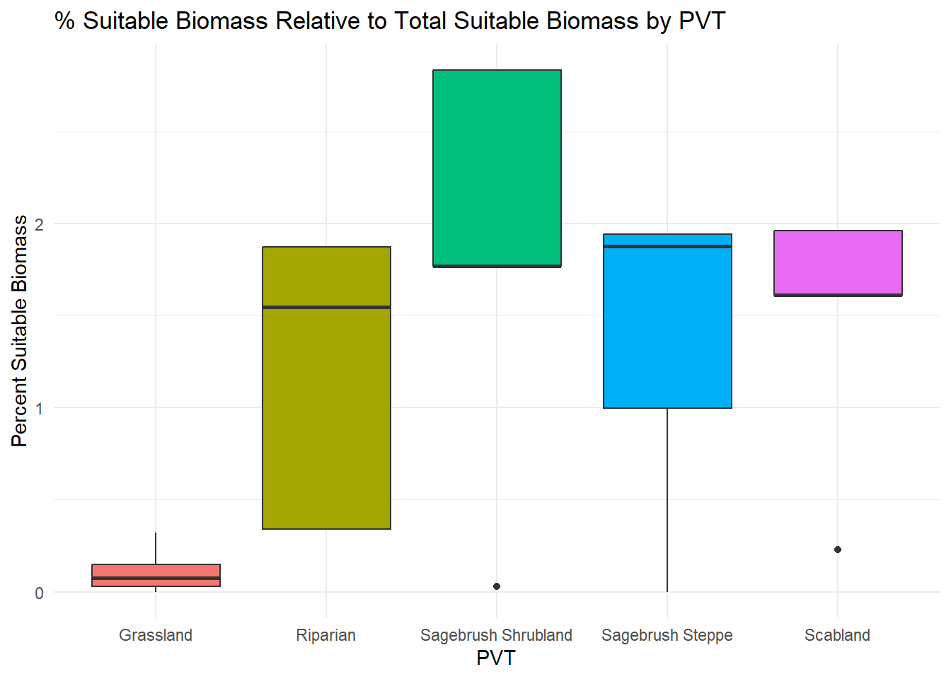
Suitable Biomass Visualizations

Code

# Calculate the percent of biomass relative to each PVT's total biomass percent
percentdata <- data %>% group_by(PVT) %>%
  mutate( total_biomass = sum(SuitableBiomass, na.rm = TRUE),  # Total biomass in each PVT 
          percent_biomass = SuitableBiomass / total_biomass * 100 # Percent biomass relative to total biomass in PVT
          ) %>% ungroup() 

# Boxplot for percent biomass 
ggplot(percentdata, aes(x = PVT, y = percent_biomass, fill = PVT)) +
  geom_boxplot() + 
  labs(title = "% Suitable Biomass Relative to Total Suitable Biomass by PVT", x = "PVT", y = "Percent Suitable Biomass") + 
  theme_minimal() + theme(legend.position = "none")

DE Visualizations

DP Visualizations

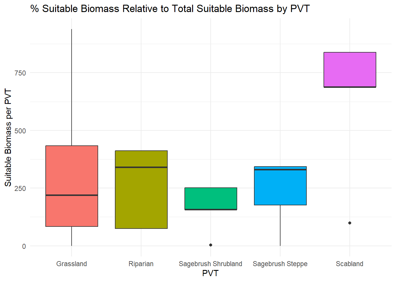
Code

# Create the boxplot
ggplot(data, aes(x = PVT, y = SuitableBiomass, fill = PVT)) + 
  geom_boxplot() + 
  labs(title = "% Suitable Biomass Relative to Total Suitable Biomass by PVT", x = "PVT", y = "Suitable Biomass per PVT") +
  theme_minimal() + 
  theme(legend.position = "none")