Checking Bio Predict Assumptions

This document contains assumption tests and plots to analyze my linear regression equations for biomass predictions.
Author

Alexis Means

Published

October 2, 2025

Code
spp_model <- readRDS("C:/Users/Alexis Means/Documents/Project/Nutrition Sampling/R code/biomass/regression_equations/24and25-Biomass-Regression-Species-Top-Model-List.rds")

fam_model <- readRDS("C:/Users/Alexis Means/Documents/Project/Nutrition Sampling/R code/biomass/regression_equations/24and25-Biomass-Regression-Family-Top-Model-List.rds")

genus_model <- readRDS("C:/Users/Alexis Means/Documents/Project/Nutrition Sampling/R code/biomass/regression_equations/24and25-Biomass-Regression-Genus-Top-Model-List.rds")

fg_model <- readRDS("C:/Users/Alexis Means/Documents/Project/Nutrition Sampling/R code/biomass/regression_equations/24and25-Biomass-Regression-Functional-Group-Top-Model-List.rds")

all_models <- list(
  spp   = spp_model,
  fam   = fam_model,
  genus = genus_model,
  fg    = fg_model
)

Predicted Biomass Values

Here are my current predicted biomass values based on the linear equations at the bottom of the page. I didn’t include the code I used to generate them in this document, but I can send it over if you’d like to take a look. Right now, all the biomass values are in grams rather than kilograms. I’m not sure if that affects the predictions, but my plan was to scale them up to kilograms before rerunning the FRESH model.

IGNORE THIS FOR NOW

Code
library(readr)
library(readxl)
library(DT)

df <- "C:/Users/Alexis Means/Documents/Project/Nutrition Sampling/R code/biomass/24and25predictions.xlsx"

predictions <- read_excel(df, "Sheet1")

datatable(predictions, options = list(pageLength = 10))

R2, AIC and Coefficients

A lot of the r-squared values look much better. The FG results still do not look great.

Code
spp <- "C:/Users/Alexis Means/Documents/Project/Nutrition Sampling/R code/biomass/processed.data/spp_models_diagnostics.xlsx"

spp_predictions <- read_excel(spp, "Sheet1")

datatable(spp_predictions, options = list(pageLength = 10))
Code
genus <- "C:/Users/Alexis Means/Documents/Project/Nutrition Sampling/R code/biomass/processed.data/genus_models_diagnostics.xlsx"

genus_predictions <- read_excel(genus, "Sheet1")

datatable(genus_predictions, options = list(pageLength = 10))
Code
fam <- "C:/Users/Alexis Means/Documents/Project/Nutrition Sampling/R code/biomass/processed.data/family_models_diagnostics.xlsx"

fam_predictions <- read_excel(fam, "Sheet1")

datatable(fam_predictions, options = list(pageLength = 10))
Code
fg <- "C:/Users/Alexis Means/Documents/Project/Nutrition Sampling/R code/biomass/processed.data/fg_models_diagnostics.xlsx"

fg_predictions <- read_excel(fg, "Sheet1")

datatable(fg_predictions, options = list(pageLength = 10))

Assumption Test P-values

  • Breusch–Pagan test (bptest) for homoscedasticity

  • Shapiro–Wilk test for normality of residuals

  • Durbin–Watson test (dwtest) for autocorrelation

  • Cook’s distance for influential observations

I’m not sure if there are other tests that would be better to run instead. I could also use some guidance on which p-values should be considered “red flags” that suggest I need to use a different equation. I rounded everything to four decimal places to make the results easier to read, so any zeros you see are just very small values above zero

Code
library(tidyverse)
library(lmtest)
library(purrr)
library(DT)

check_lm_assumptions <- function(model) {
  if (!inherits(model, "lm")) return(NULL)
  
  res <- residuals(model)
  
  list(
    r_squared = tryCatch(round(summary(model)$r.squared, 4), error = function(e) NA),
    shapiro_p = tryCatch(round(shapiro.test(res)$p.value, 4), error = function(e) NA),
    bp_test   = tryCatch(round(lmtest::bptest(model)$p.value, 4), error = function(e) NA),
    dw_test   = tryCatch(round(lmtest::dwtest(model)$p.value, 4), error = function(e) NA),
    cook_max  = tryCatch(round(max(cooks.distance(model), na.rm = TRUE), 4), error = function(e) NA)
  )
}

diagnostics <- imap_dfr(all_models, function(model_list, group_name) {
  map_dfr(model_list, check_lm_assumptions, .id = "model_name") %>%
    mutate(group = group_name, .before = 1)
})

#--------------------------------------------------------------
# 3️⃣ Extract model base name (everything before trailing number)
#     Example: "BRTE_GREEN1" → "BRTE_GREEN"
#--------------------------------------------------------------
diagnostics <- diagnostics %>%
  mutate(model_base = str_trim(str_extract(model_name, ".*(?=\\d+$)")))

#--------------------------------------------------------------
# 4️⃣ Identify and remove model families with any R² > 0.4
#--------------------------------------------------------------
high_r2_bases <- diagnostics %>%
  group_by(model_base) %>%
  summarize(any_high_r2 = any(r_squared > 0.4, na.rm = TRUE)) %>%
  filter(any_high_r2) %>%
  pull(model_base)

diagnostics_low_r2 <- diagnostics %>%
  filter(!model_base %in% high_r2_bases)


datatable(diagnostics_low_r2, options = list(pageLength = 10))

Diagnostic Plots and Equations

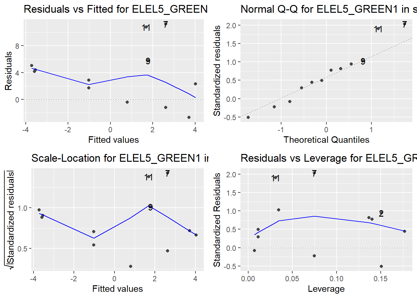
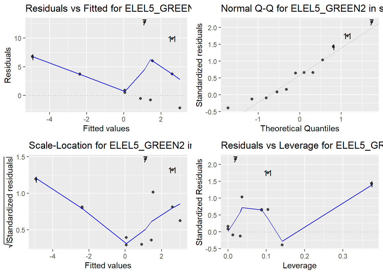
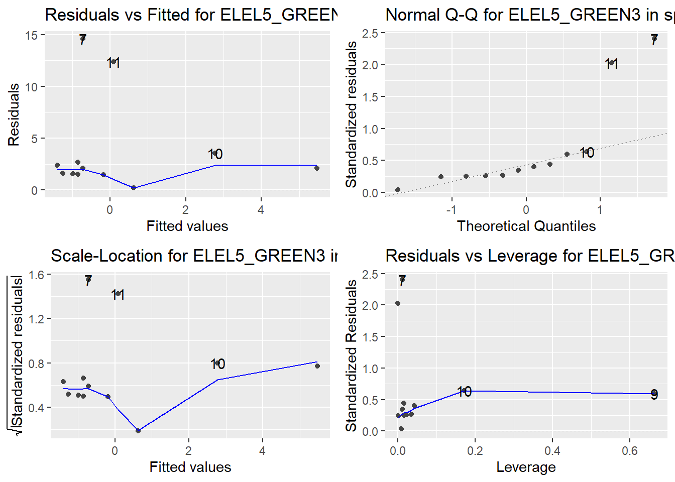
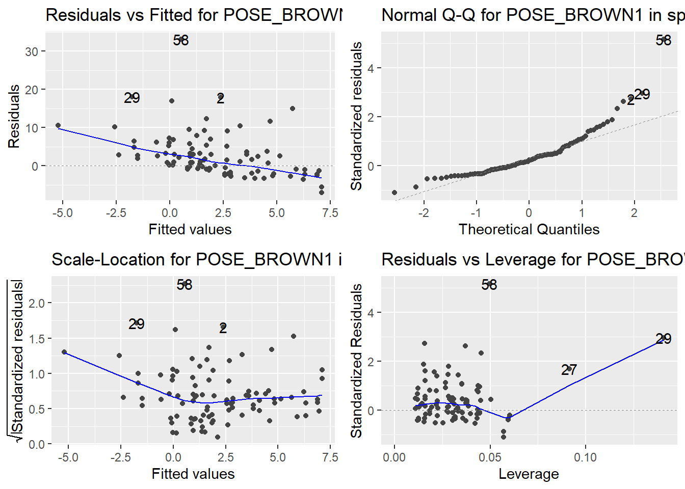
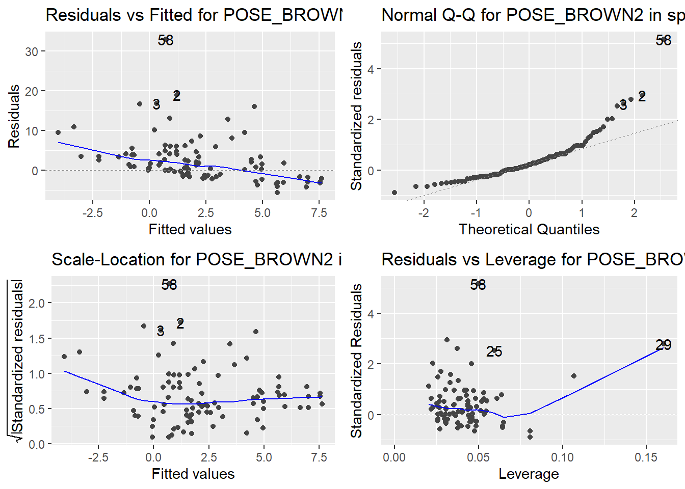
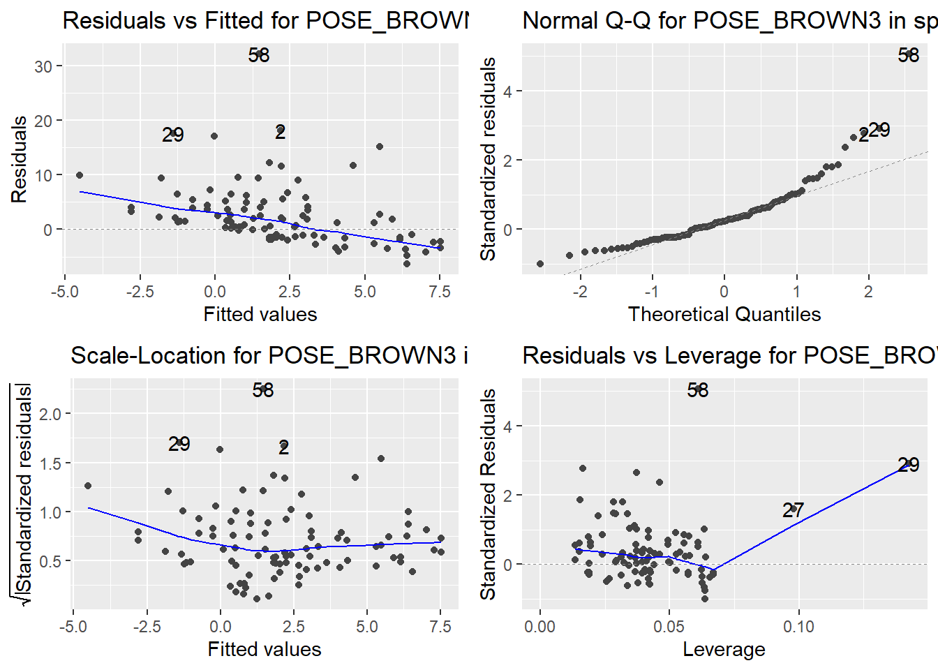
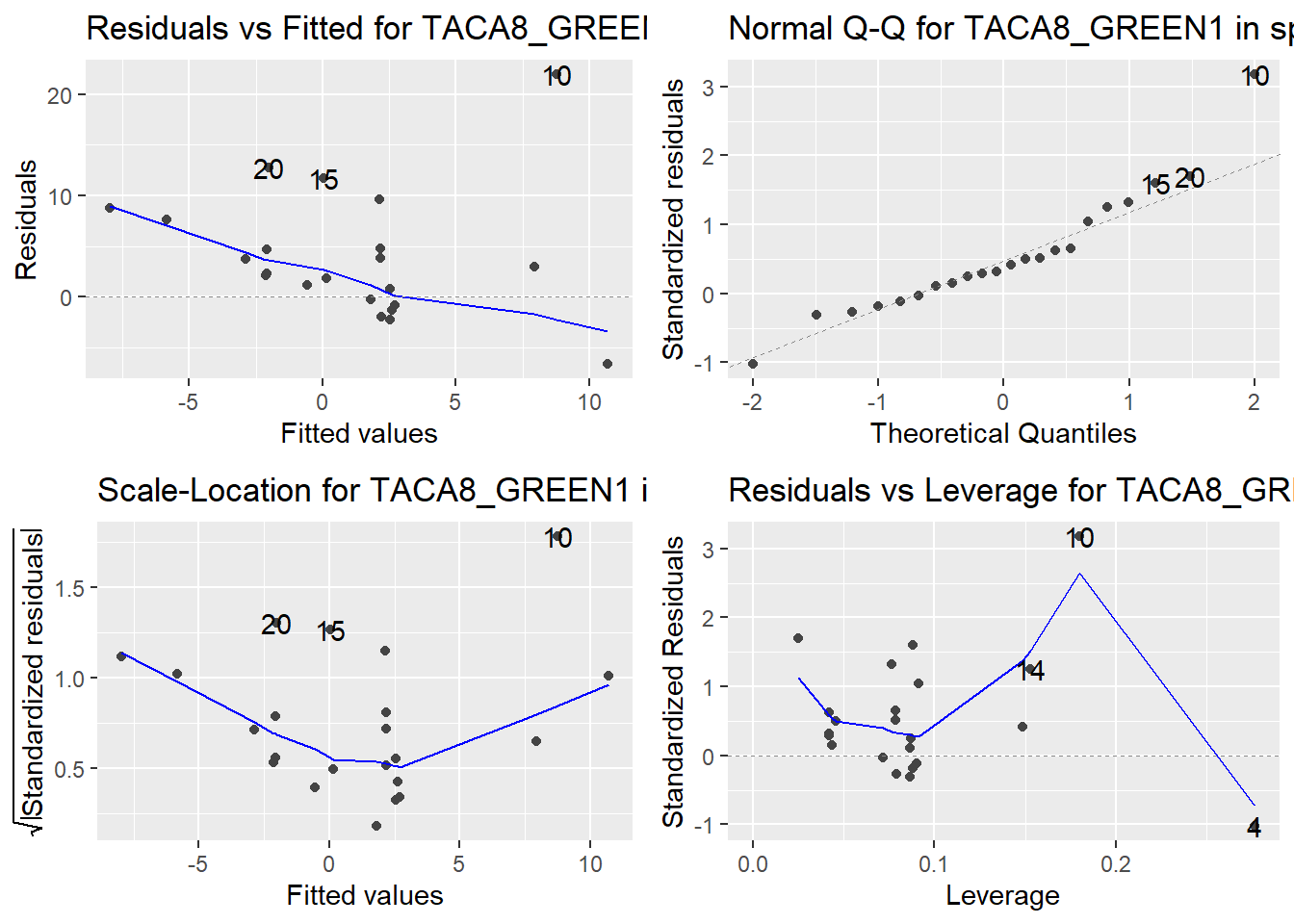
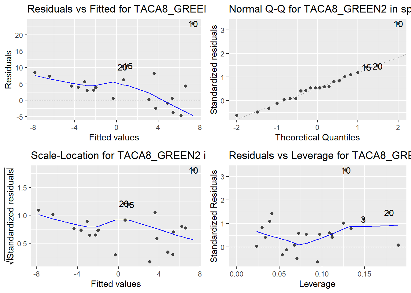
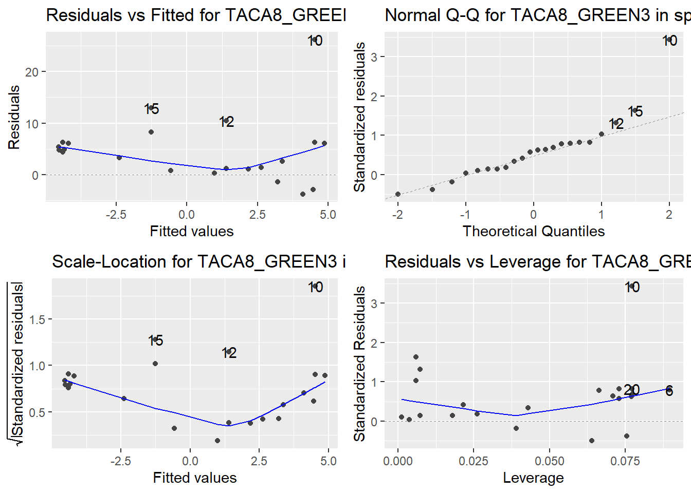
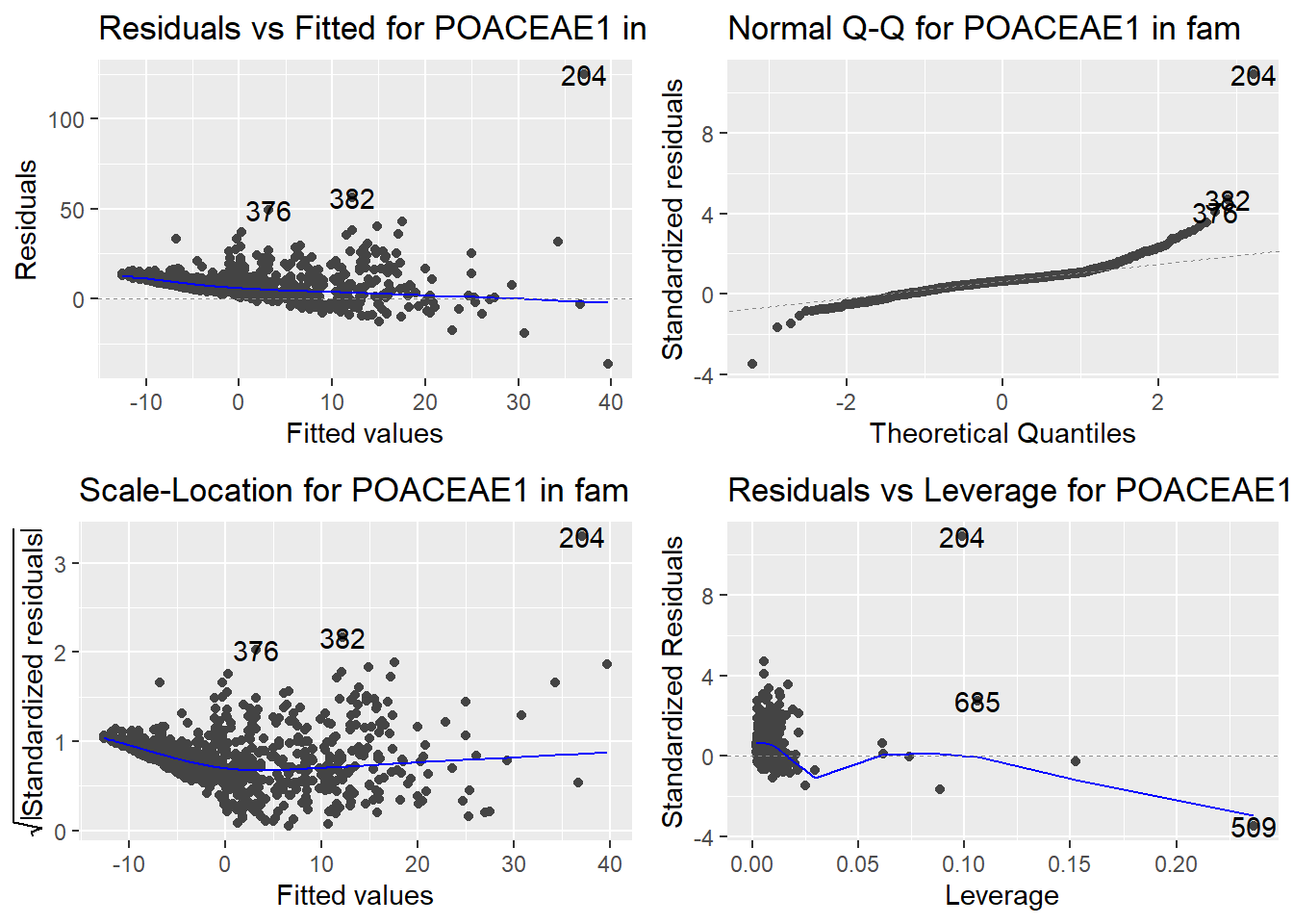
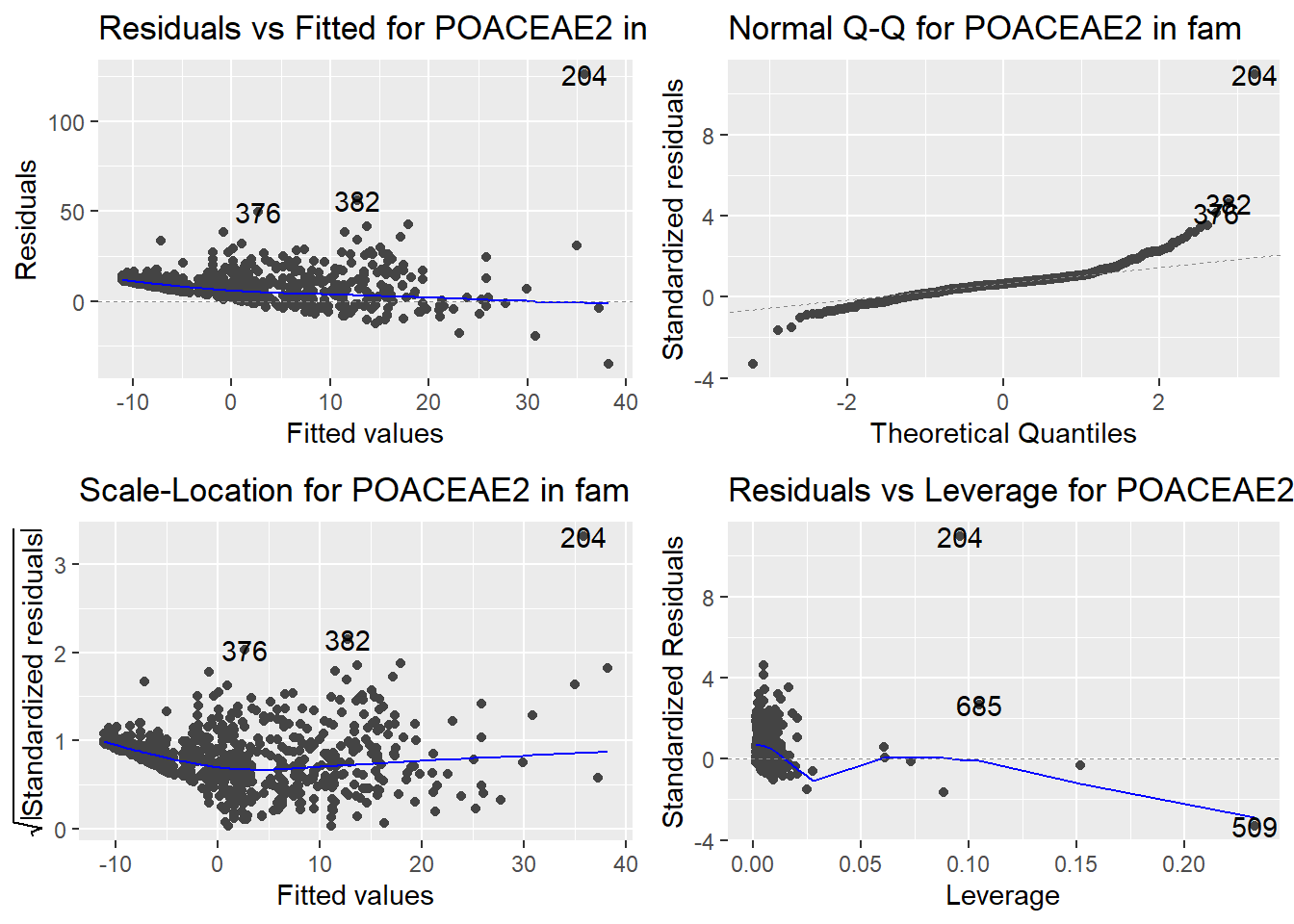
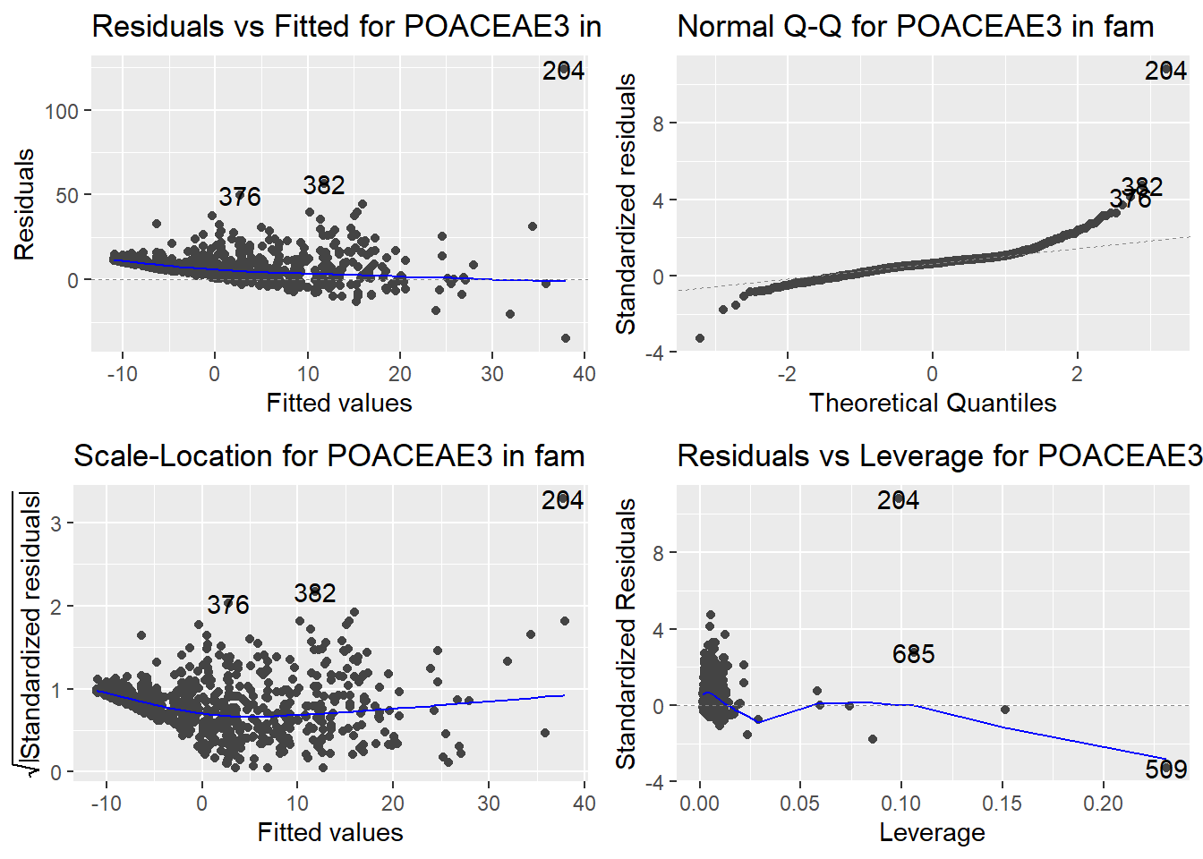
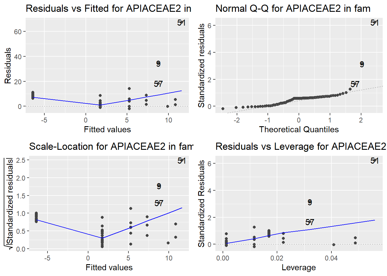
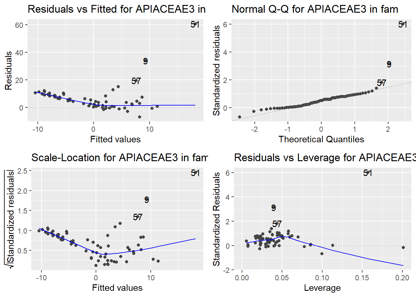
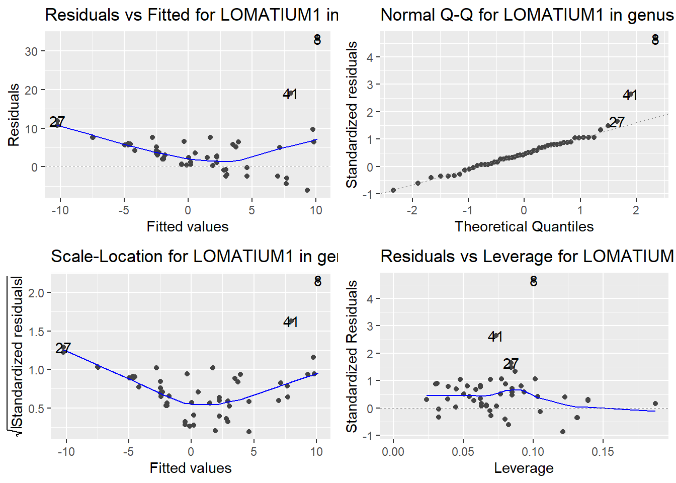
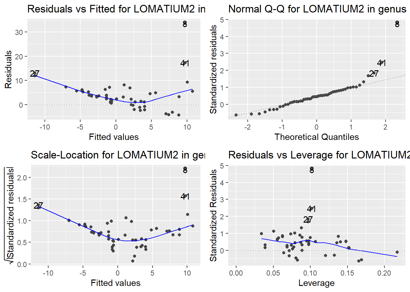
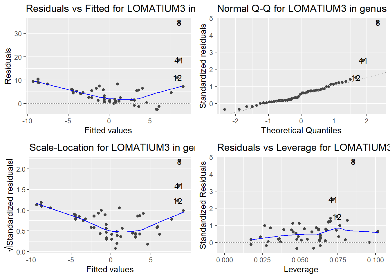
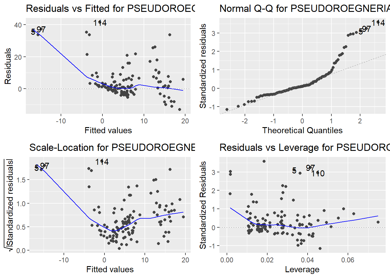
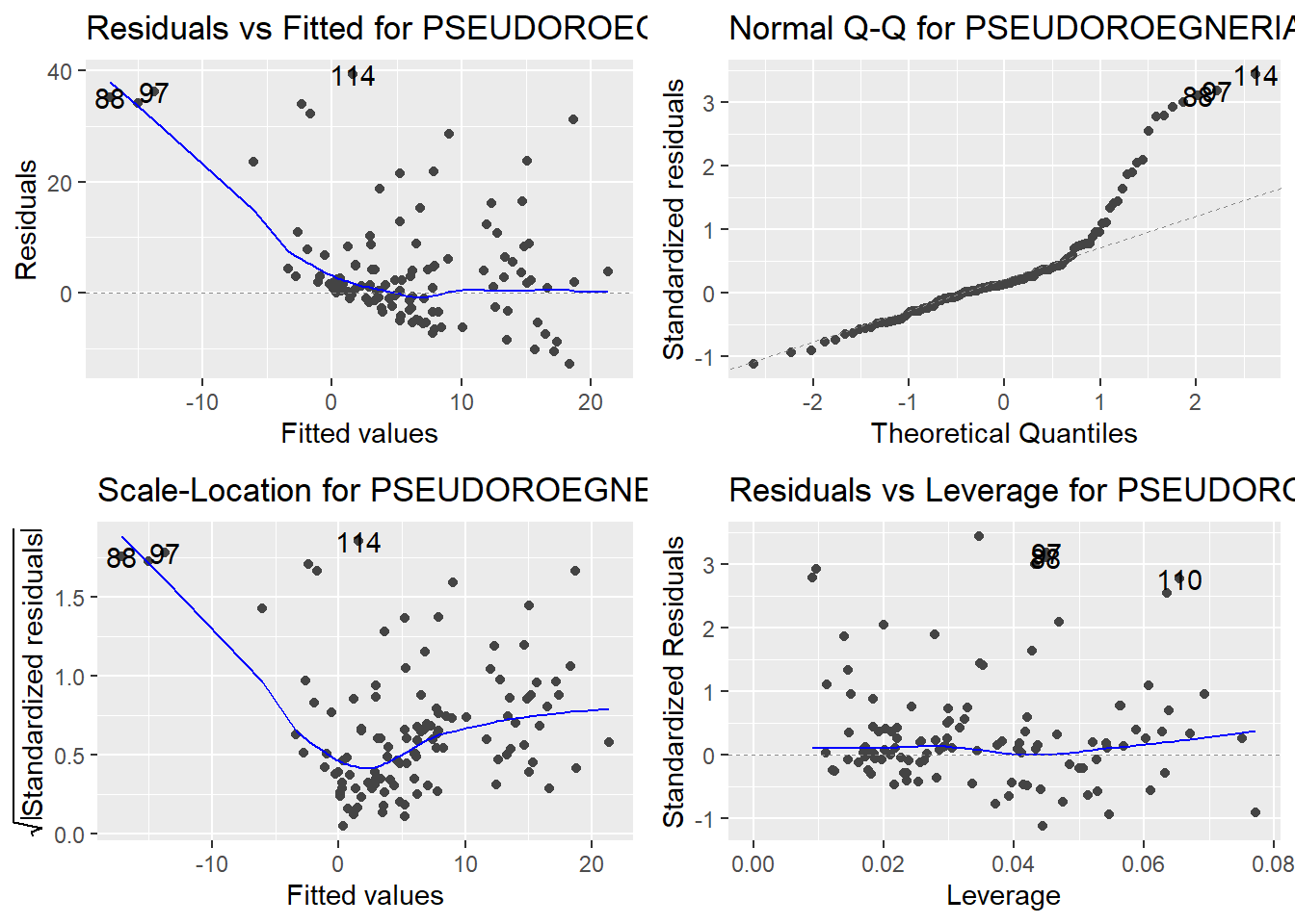
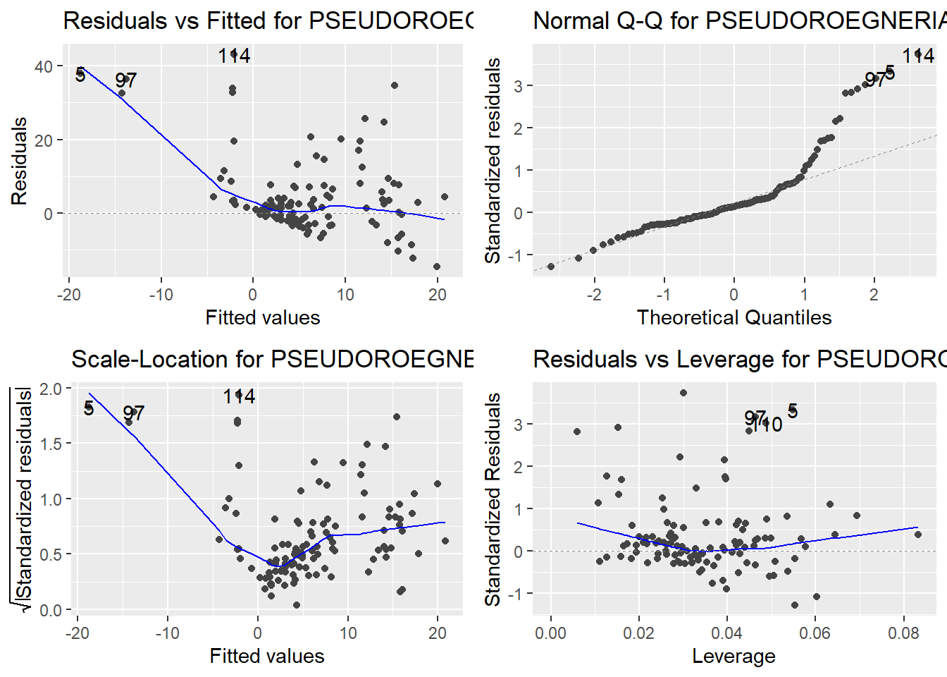
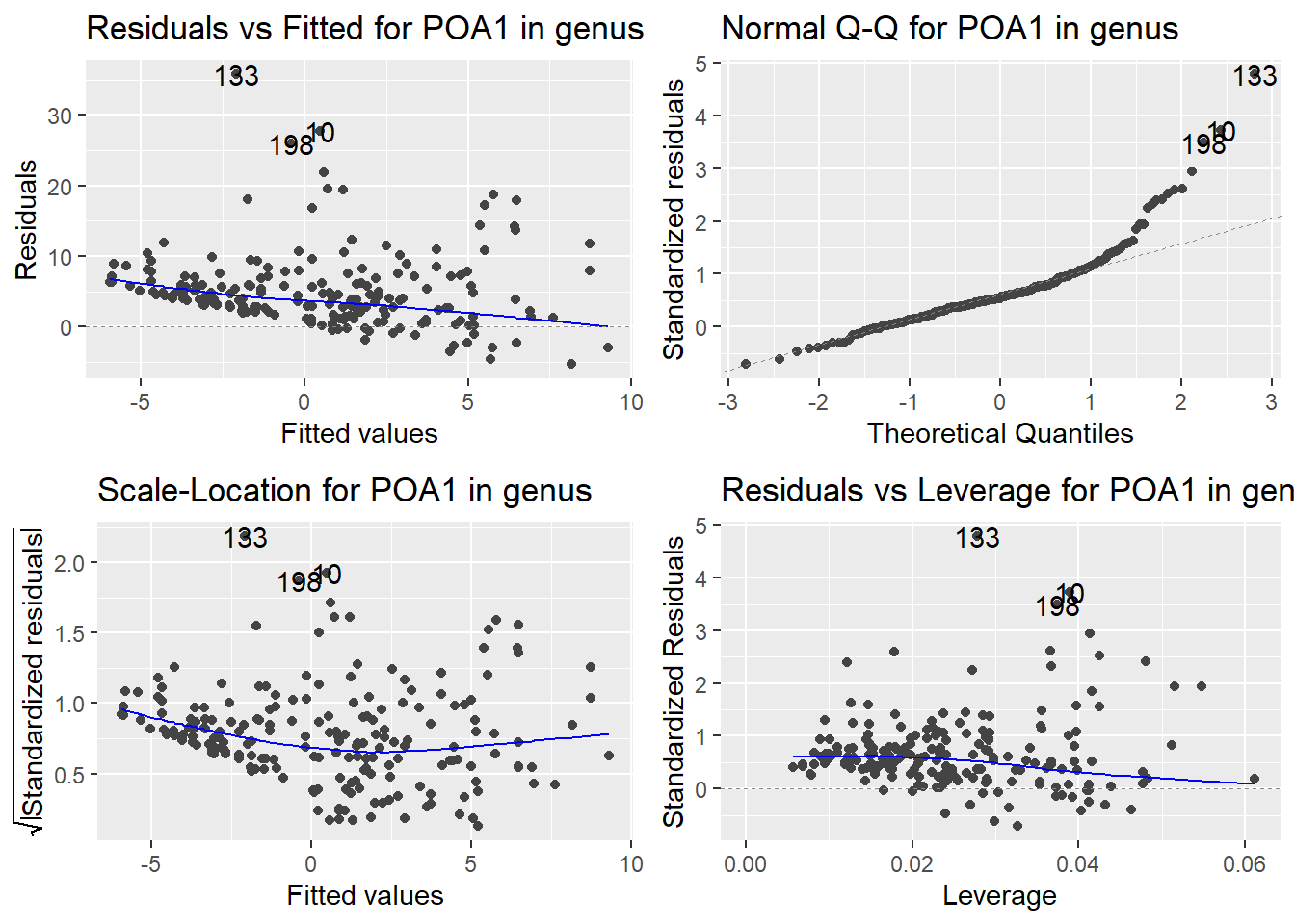
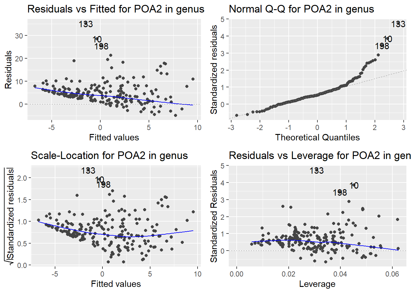
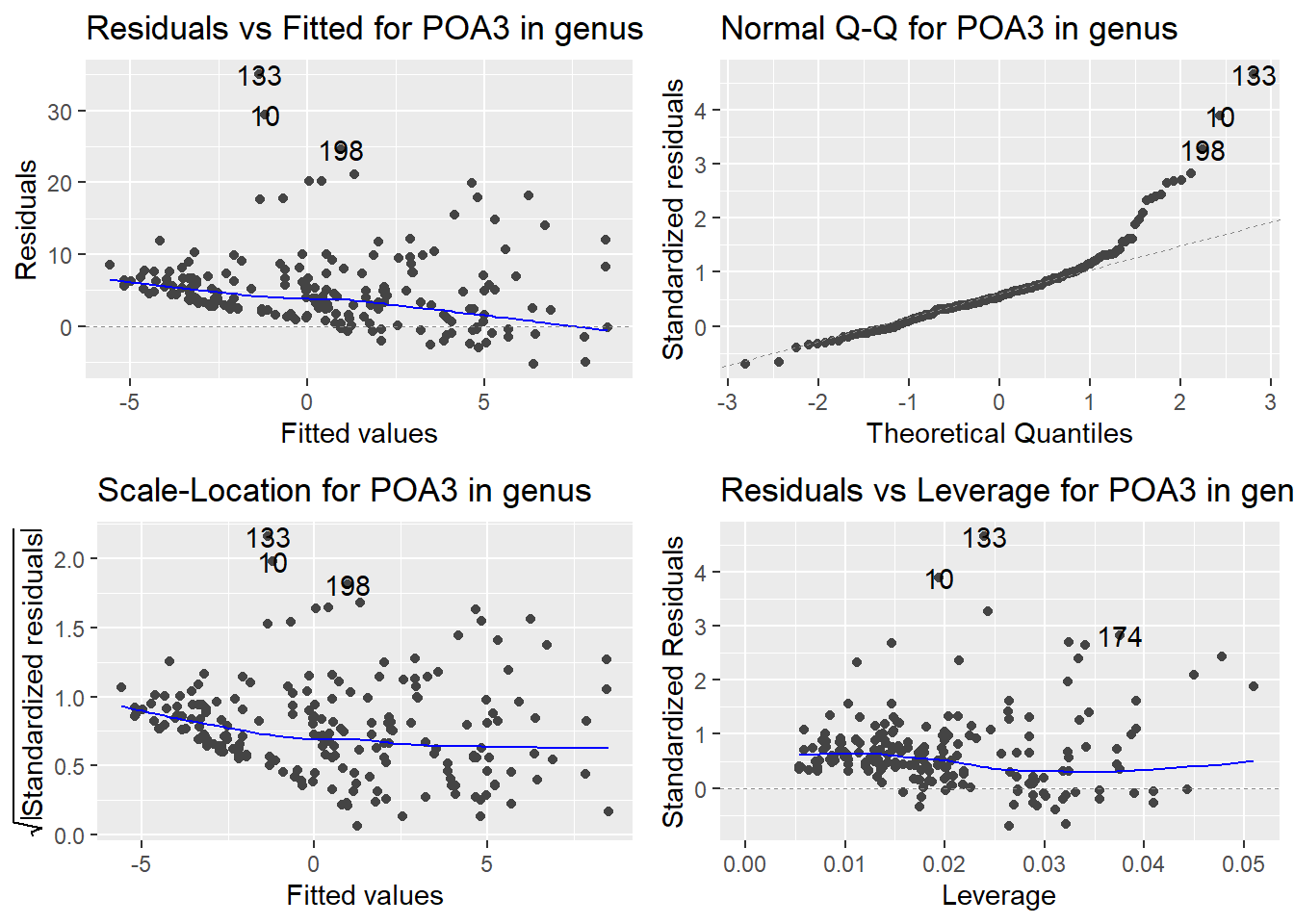
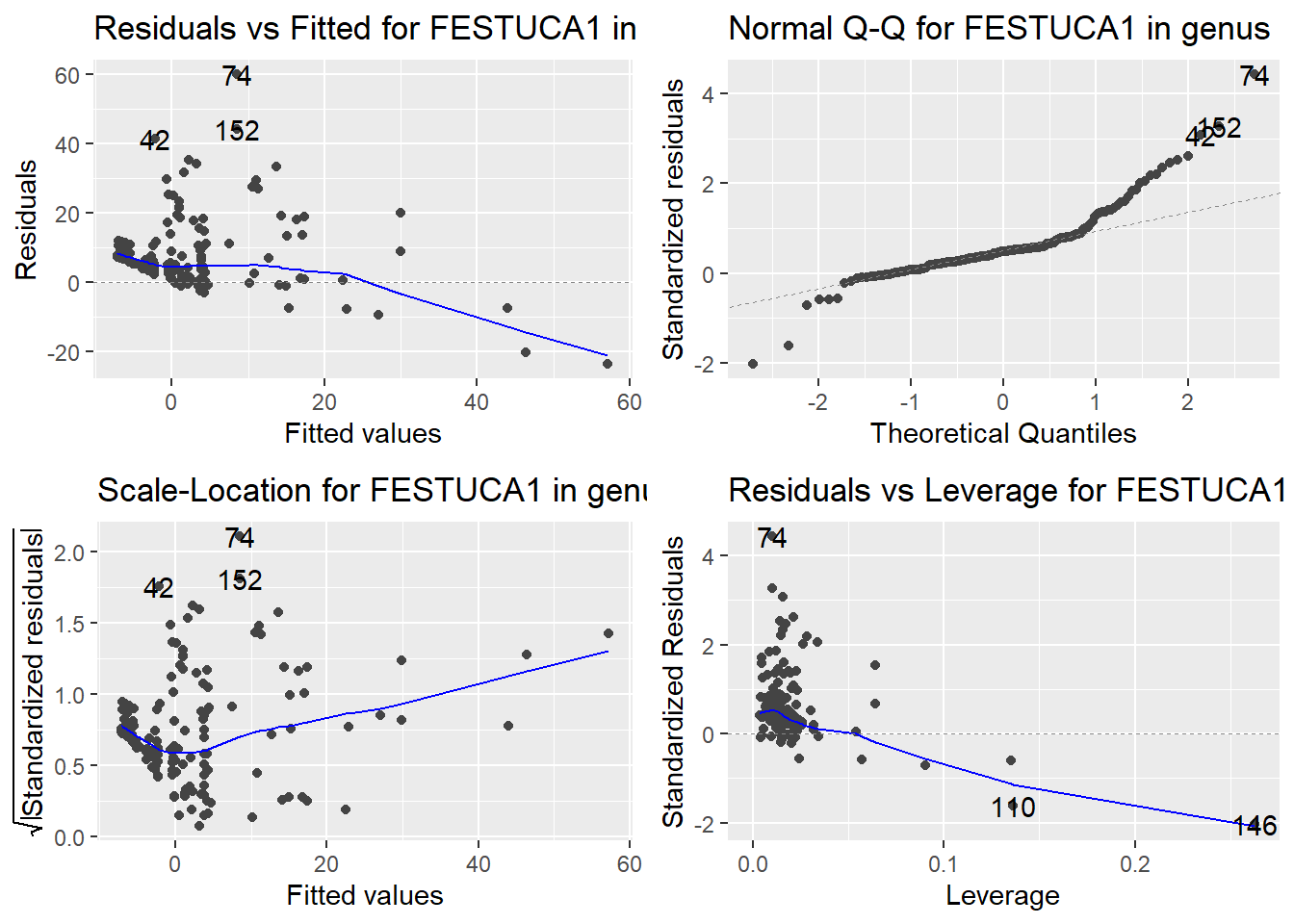
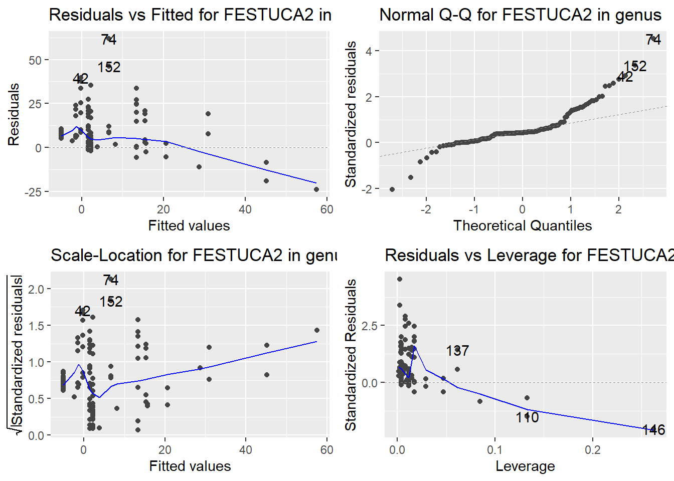
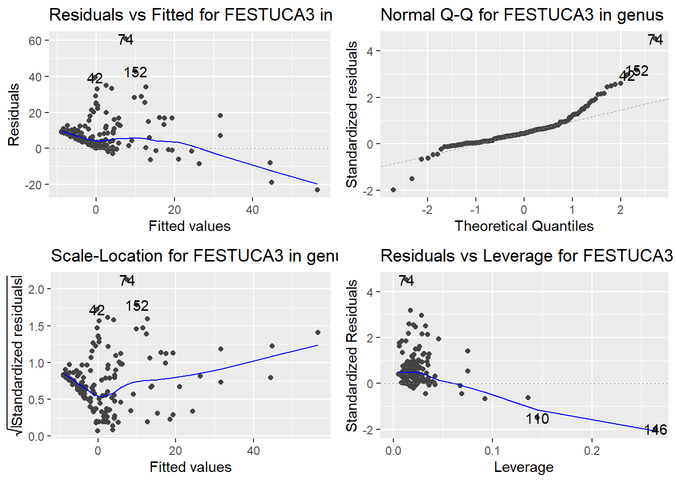
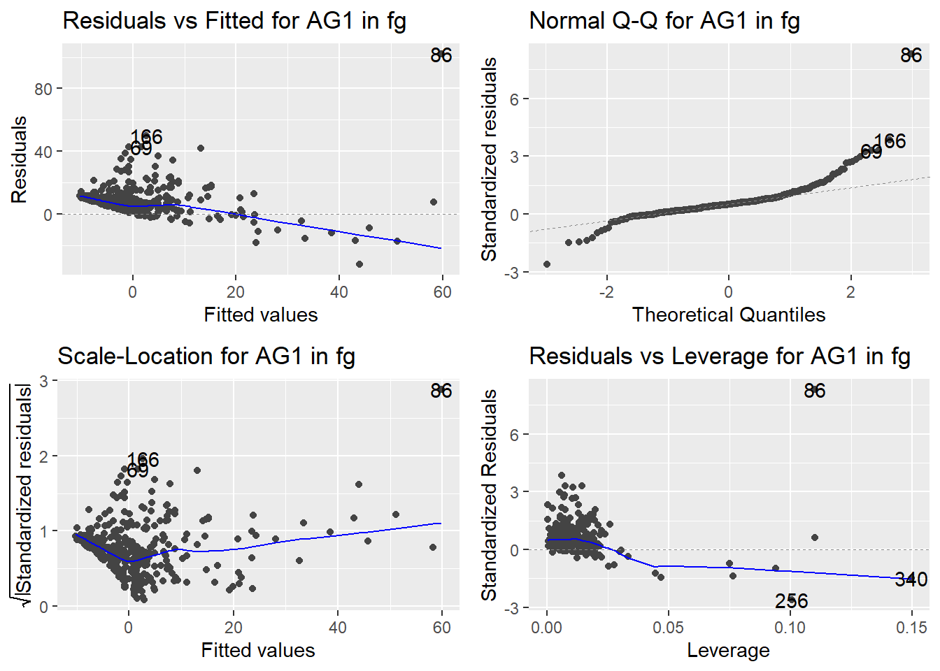
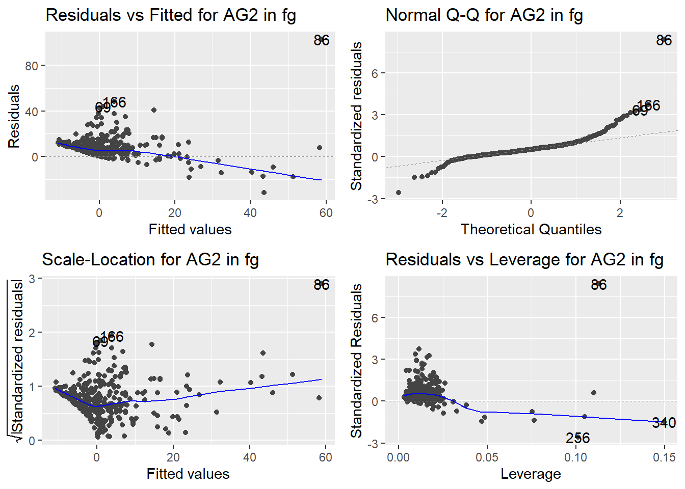
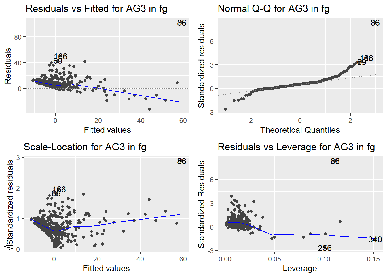
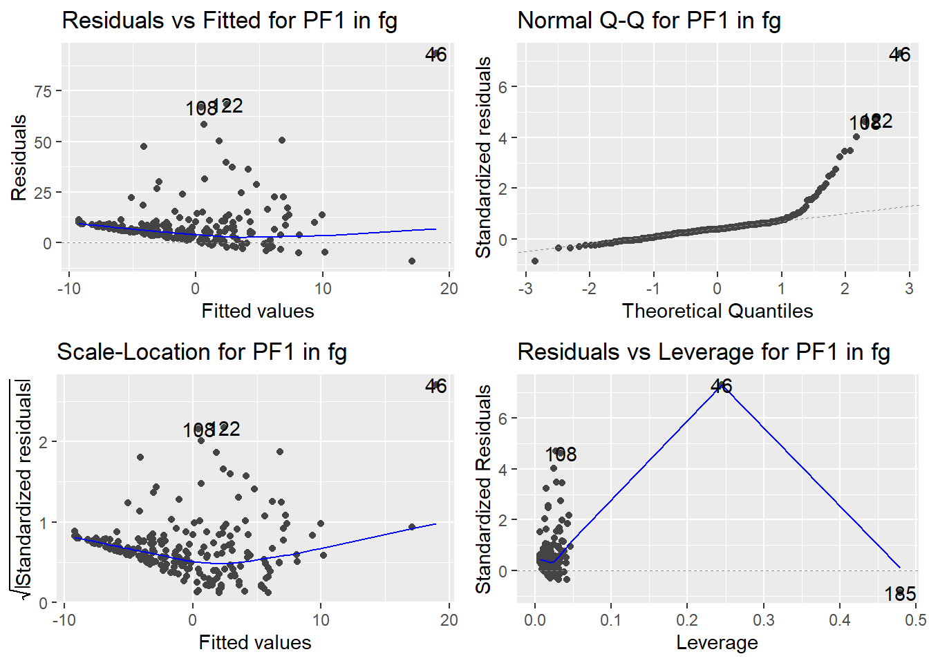
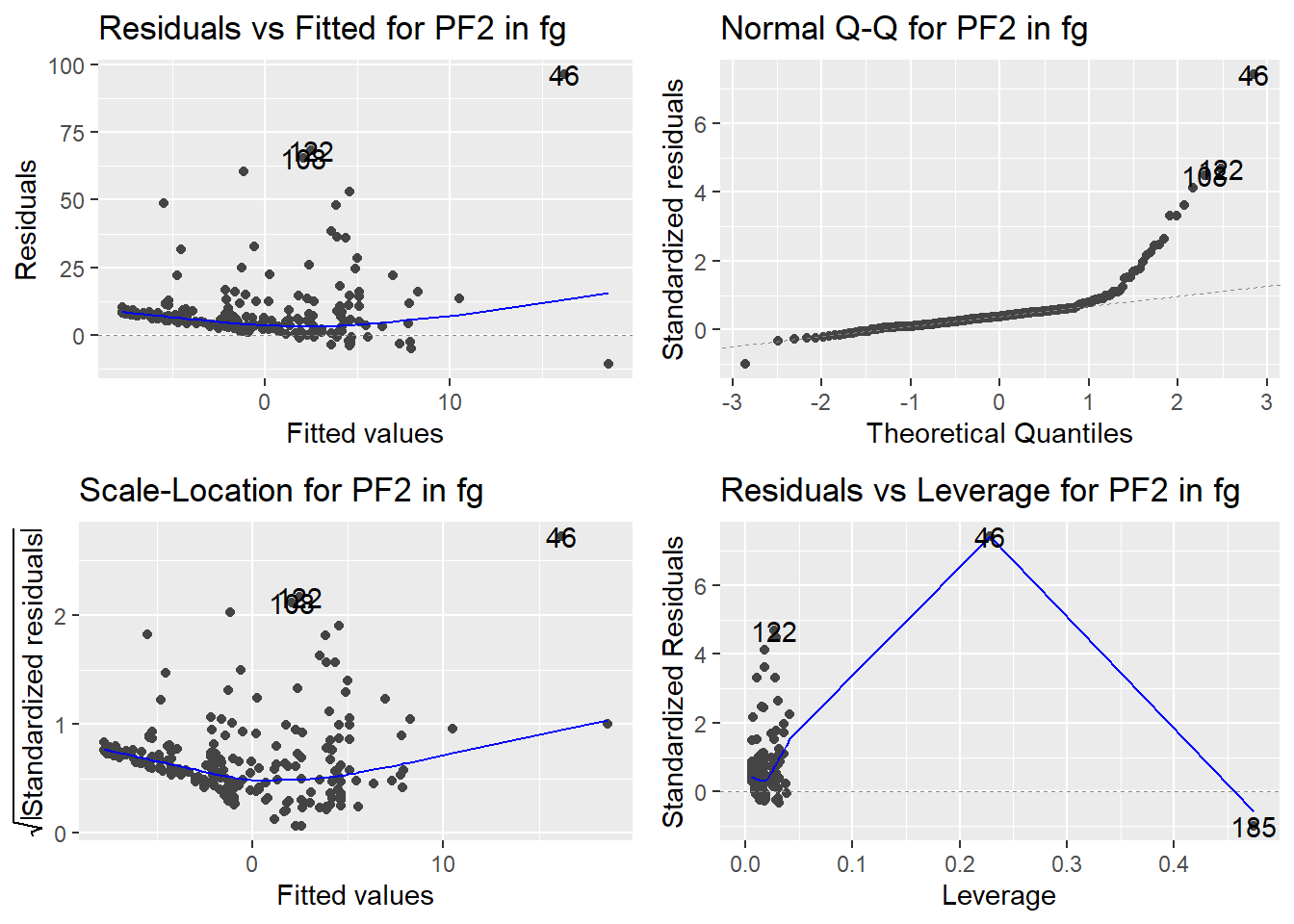
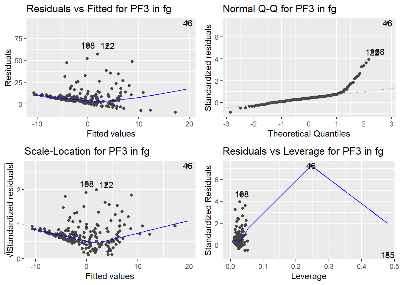
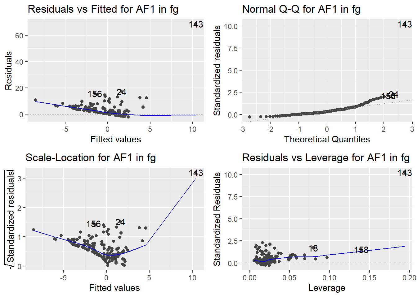
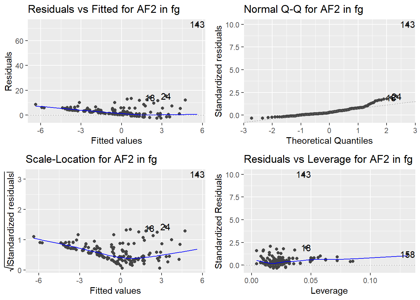
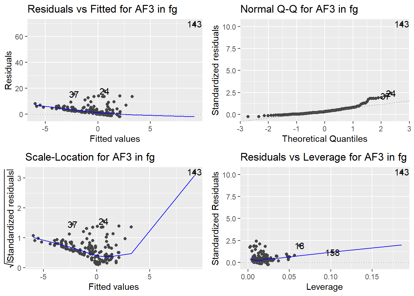
Here are the diagnostic plots for each of the linear models: Breusch–Pagan test (top left), Shapiro–Wilk test (top right), Durbin–Watson test (bottom left), and Cook’s distance (bottom right). Below the plots, I’ve also included each of the linear equations I’m using to predict biomass.

Code
library(ggfortify)
library(gridExtra)

plot_diagnostics <- function(model, model_name, group_name) {
  
  p1 <- autoplot(model, which = 1)[[1]] + 
    ggtitle(paste("Residuals vs Fitted for", model_name, "in", group_name))
  
  p2 <- autoplot(model, which = 2)[[1]] + 
    ggtitle(paste("Normal Q-Q for", model_name, "in", group_name))
  
  p3 <- autoplot(model, which = 3)[[1]] + 
    ggtitle(paste("Scale-Location for", model_name, "in", group_name))
  
  p4 <- autoplot(model, which = 5)[[1]] + 
    ggtitle(paste("Residuals vs Leverage for", model_name, "in", group_name))
  
  gridExtra::grid.arrange(p1, p2, p3, p4, ncol = 2)
}

imap(all_models, function(model_list, group_name) {
  
  # Filter only models from this group that passed the R² criteria
  keep_models <- diagnostics_low_r2 %>%
    filter(group == group_name) %>%
    pull(model_name)
  
  # Subset model list to those models
  model_list_filtered <- model_list[names(model_list) %in% keep_models]
  
  # Plot only the retained models
  walk2(model_list_filtered, names(model_list_filtered), ~ {
    plot_diagnostics(.x, .y, group_name)
  })
})

$spp
$spp$ELEL5_GREEN1

Call:
lm(formula = y ~ 0 + Abiotic.cover_sin, data = z, na.action = na.fail)

Coefficients:
Abiotic.cover_sin  
            2.758  


$spp$ELEL5_GREEN2

Call:
lm(formula = y ~ 0 + julian_identity, data = z, na.action = na.fail)

Coefficients:
julian_identity  
          3.276  


$spp$ELEL5_GREEN3

Call:
lm(formula = y ~ 0 + Abiotic.cover_identity, data = z, na.action = na.fail)

Coefficients:
Abiotic.cover_identity  
                -2.712  


$spp$POSE_BROWN1

Call:
lm(formula = y ~ 0 + elev_sqrt + julian_cos + Percent_cubic, 
    data = z, na.action = na.fail)

Coefficients:
    elev_sqrt     julian_cos  Percent_cubic  
        2.487         -1.730        -11.852  


$spp$POSE_BROWN2

Call:
lm(formula = y ~ 0 + elev_sqrt + julian_cos + Percent_cubic + 
    Percent_sin, data = z, na.action = na.fail)

Coefficients:
    elev_sqrt     julian_cos  Percent_cubic    Percent_sin  
       2.2715        -1.6034       -10.9962        -0.9478  


$spp$POSE_BROWN3

Call:
lm(formula = y ~ 0 + elev_cos + elev_sqrt + julian_cos + Percent_cubic, 
    data = z, na.action = na.fail)

Coefficients:
     elev_cos      elev_sqrt     julian_cos  Percent_cubic  
      -0.8525         2.6713        -1.8427       -11.4857  


$spp$TACA8_GREEN1

Call:
lm(formula = y ~ 0 + elev_sin + Percent_sin, data = z, na.action = na.fail)

Coefficients:
   elev_sin  Percent_sin  
     -4.237       -3.660  


$spp$TACA8_GREEN2

Call:
lm(formula = y ~ 0 + Abiotic.cover_sin + elev_sqrt, data = z, 
    na.action = na.fail)

Coefficients:
Abiotic.cover_sin          elev_sqrt  
            3.404              2.180  


$spp$TACA8_GREEN3

Call:
lm(formula = y ~ 0 + Abiotic.cover_sin, data = z, na.action = na.fail)

Coefficients:
Abiotic.cover_sin  
            3.379  


$fam
$fam$POACEAE1

Call:
lm(formula = y ~ 0 + asp_cos + elev_sin + julian_quadratic + 
    Percent_cubic + Percent_log + Percent_sin, data = z, na.action = na.fail)

Coefficients:
         asp_cos          elev_sin  julian_quadratic     Percent_cubic  
          0.8994           -1.8047            0.8842            1.7495  
     Percent_log       Percent_sin  
          8.6610            1.7472  


$fam$POACEAE2

Call:
lm(formula = y ~ 0 + elev_sin + julian_quadratic + Percent_cubic + 
    Percent_log + Percent_sin, data = z, na.action = na.fail)

Coefficients:
        elev_sin  julian_quadratic     Percent_cubic       Percent_log  
         -1.7301            0.6619            1.7303            8.6194  
     Percent_sin  
          1.7355  


$fam$POACEAE3

Call:
lm(formula = y ~ 0 + asp_cos + elev_sin + Percent_cubic + Percent_log + 
    Percent_sin, data = z, na.action = na.fail)

Coefficients:
      asp_cos       elev_sin  Percent_cubic    Percent_log    Percent_sin  
       0.6712        -1.8542         1.8303         8.5696         1.7916  


$fam$APIACEAE1

Call:
lm(formula = y ~ 0 + Abiotic.cover_log + Percent_log, data = z, 
    na.action = na.fail)

Coefficients:
Abiotic.cover_log        Percent_log  
           -2.338              6.181  


$fam$APIACEAE2

Call:
lm(formula = y ~ 0 + Percent_log, data = z, na.action = na.fail)

Coefficients:
Percent_log  
      6.177  


$fam$APIACEAE3

Call:
lm(formula = y ~ 0 + Abiotic.cover_log + Abiotic.cover_sin + 
    Percent_log, data = z, na.action = na.fail)

Coefficients:
Abiotic.cover_log  Abiotic.cover_sin        Percent_log  
           -2.266              1.283              6.262  


$genus
$genus$LOMATIUM1

Call:
lm(formula = y ~ 0 + asp_sin + julian_sin + julian_sqrt + Percent_log, 
    data = z, na.action = na.fail)

Coefficients:
    asp_sin   julian_sin  julian_sqrt  Percent_log  
     -2.913        1.789       -2.026        3.583  


$genus$LOMATIUM2

Call:
lm(formula = y ~ 0 + asp_sin + julian_cos + julian_sin + julian_sqrt + 
    Percent_log, data = z, na.action = na.fail)

Coefficients:
    asp_sin   julian_cos   julian_sin  julian_sqrt  Percent_log  
     -2.464        1.587        1.753       -2.302        3.665  


$genus$LOMATIUM3

Call:
lm(formula = y ~ 0 + asp_sin + julian_sin + Percent_log, data = z, 
    na.action = na.fail)

Coefficients:
    asp_sin   julian_sin  Percent_log  
     -2.286        1.827        3.929  


$genus$PSEUDOROEGNERIA1

Call:
lm(formula = y ~ 0 + Abiotic.cover_quadratic + Percent_cos + 
    Percent_cubic, data = z, na.action = na.fail)

Coefficients:
Abiotic.cover_quadratic              Percent_cos            Percent_cubic  
                 -2.093                   -5.282                  -40.407  


$genus$PSEUDOROEGNERIA2

Call:
lm(formula = y ~ 0 + Abiotic.cover_quadratic + elev_sqrt + Percent_cos + 
    Percent_cubic, data = z, na.action = na.fail)

Coefficients:
Abiotic.cover_quadratic                elev_sqrt              Percent_cos  
                 -2.198                    1.698                   -5.251  
          Percent_cubic  
                -40.222  


$genus$PSEUDOROEGNERIA3

Call:
lm(formula = y ~ 0 + Abiotic.cover_quadratic + elev_sin + Percent_cos + 
    Percent_cubic, data = z, na.action = na.fail)

Coefficients:
Abiotic.cover_quadratic                 elev_sin              Percent_cos  
                 -1.909                   -1.246                   -5.401  
          Percent_cubic  
                -40.570  


$genus$POA1

Call:
lm(formula = y ~ 0 + elev_cubic + julian_cos + julian_log + Percent_cos + 
    Percent_sin, data = z, na.action = na.fail)

Coefficients:
 elev_cubic   julian_cos   julian_log  Percent_cos  Percent_sin  
     1.6742      -1.1443      -0.8561      -1.9497      -1.3449  


$genus$POA2

Call:
lm(formula = y ~ 0 + Abiotic.cover_cos + elev_cubic + julian_cos + 
    julian_log + Percent_cos + Percent_sin, data = z, na.action = na.fail)

Coefficients:
Abiotic.cover_cos         elev_cubic         julian_cos         julian_log  
          -0.7336             1.7124            -1.1339            -0.8708  
      Percent_cos        Percent_sin  
          -1.8615            -1.3250  


$genus$POA3

Call:
lm(formula = y ~ 0 + elev_cubic + julian_cos + Percent_cos + 
    Percent_sin, data = z, na.action = na.fail)

Coefficients:
 elev_cubic   julian_cos  Percent_cos  Percent_sin  
      1.601       -1.115       -2.102       -1.289  


$genus$FESTUCA1

Call:
lm(formula = y ~ 0 + asp_sin + Percent_quadratic + Percent_sin, 
    data = z, na.action = na.fail)

Coefficients:
          asp_sin  Percent_quadratic        Percent_sin  
            1.753              7.016             -2.898  


$genus$FESTUCA2

Call:
lm(formula = y ~ 0 + Percent_quadratic + Percent_sin, data = z, 
    na.action = na.fail)

Coefficients:
Percent_quadratic        Percent_sin  
            7.165             -3.172  


$genus$FESTUCA3

Call:
lm(formula = y ~ 0 + asp_sin + elev_sin + Percent_quadratic + 
    Percent_sin, data = z, na.action = na.fail)

Coefficients:
          asp_sin           elev_sin  Percent_quadratic        Percent_sin  
            1.750             -1.328              7.047             -2.933  


$fg
$fg$AG1

Call:
lm(formula = y ~ 0 + asp_cos + elev_sin + Percent_cos + Percent_quadratic, 
    data = z, na.action = na.fail)

Coefficients:
          asp_cos           elev_sin        Percent_cos  Percent_quadratic  
            1.860             -2.901             -2.740              6.885  


$fg$AG2

Call:
lm(formula = y ~ 0 + asp_cos + elev_sin + Percent_cos + Percent_quadratic + 
    Percent_sin, data = z, na.action = na.fail)

Coefficients:
          asp_cos           elev_sin        Percent_cos  Percent_quadratic  
            1.798             -2.915             -2.413              6.955  
      Percent_sin  
           -1.014  


$fg$AG3

Call:
lm(formula = y ~ 0 + asp_cos + elev_log + elev_sin + Percent_cos + 
    Percent_quadratic, data = z, na.action = na.fail)

Coefficients:
          asp_cos           elev_log           elev_sin        Percent_cos  
           1.9704            -0.7723            -2.9152            -2.7284  
Percent_quadratic  
           6.8513  


$fg$PF1

Call:
lm(formula = y ~ 0 + Abiotic.cover_cos + elev_cos + Percent_cos + 
    Percent_cubic + Percent_sin, data = z, na.action = na.fail)

Coefficients:
Abiotic.cover_cos           elev_cos        Percent_cos      Percent_cubic  
            2.600             -1.436             -2.134              8.177  
      Percent_sin  
           -1.962  


$fg$PF2

Call:
lm(formula = y ~ 0 + Abiotic.cover_cos + Percent_cos + Percent_cubic + 
    Percent_sin, data = z, na.action = na.fail)

Coefficients:
Abiotic.cover_cos        Percent_cos      Percent_cubic        Percent_sin  
            2.388             -2.132              7.975             -2.060  


$fg$PF3

Call:
lm(formula = y ~ 0 + Abiotic.cover_cos + asp_sin + elev_cos + 
    Percent_cos + Percent_cubic + Percent_sin, data = z, na.action = na.fail)

Coefficients:
Abiotic.cover_cos            asp_sin           elev_cos        Percent_cos  
            2.568              1.350             -1.483             -2.342  
    Percent_cubic        Percent_sin  
            7.747             -1.941  


$fg$AF1

Call:
lm(formula = y ~ 0 + Abiotic.cover_cubic + elev_cos + julian_cubic + 
    Percent_cubic, data = z, na.action = na.fail)

Coefficients:
Abiotic.cover_cubic             elev_cos         julian_cubic  
             -1.261                1.242               -1.257  
      Percent_cubic  
              7.812  


$fg$AF2

Call:
lm(formula = y ~ 0 + Abiotic.cover_cubic + elev_cos + julian_cubic + 
    Percent_log, data = z, na.action = na.fail)

Coefficients:
Abiotic.cover_cubic             elev_cos         julian_cubic  
             -1.152                1.210               -1.190  
        Percent_log  
              1.342  


$fg$AF3

Call:
lm(formula = y ~ 0 + Abiotic.cover_cubic + elev_cos + Percent_cubic, 
    data = z, na.action = na.fail)

Coefficients:
Abiotic.cover_cubic             elev_cos        Percent_cubic  
             -1.394                1.157                6.609  

Questions

  1. I’m having a hard time figuring out which plots are bad enough that they justify trying a different linear model. Did any of them stick out to you?

  2. Are there any assumption tests that I should be taking with a grain of salt? Ryan mentioned that one of them might not matter as much since our main goal with the linear models is prediction.

  3. Currently, I only have the top regression equation saved for each species, genus, etc. Before I go back and rerun the model dredging process to generate more equations, I wanted to check if you had any other suggestions on how I could improve the predictions.